熟悉 Tidymodels

Progress

Learning Progress: Completed.😸

Learning Source

• https://www.tidymodels.org/

1 tidymodels 中的包

library(tidymodels)
library(tidyverse)

1.1 rsample

官网：https://rsample.tidymodels.org/

1.1.1 Index

library(mlbench)

data("LetterRecognition")
lobstr::obj_size(LetterRecognition)
#> 2.64 MB

set.seed(35222)
boots <- bootstraps(LetterRecognition, times = 50)
lobstr::obj_size(boots)
#> 6.69 MB

# Object size per resample
lobstr::obj_size(boots) / nrow(boots)
#> 133.74 kB

as.numeric(lobstr::obj_size(boots)) / as.numeric(lobstr::obj_size(LetterRecognition))
#> [1] 2.528489

The memory usage for 50 bootstrap samples is less than 3-fold more than the original data set.

1.1.2 Get started

set.seed(8584)
bt_resamples <- bootstraps(mtcars, times = 3)
bt_resamples
#> # Bootstrap sampling 
#> # A tibble: 3 × 2
#>   splits          id        
#>   <list>          <chr>     
#> 1 <split [32/14]> Bootstrap1
#> 2 <split [32/12]> Bootstrap2
#> 3 <split [32/14]> Bootstrap3

The resamples are stored in the splits column in an object that has class rsplit.

In this package we use the following terminology for the two partitions that comprise a resample:

• The analysis data are those that we selected in the resample. For a bootstrap, this is the sample with replacement. For 10-fold cross-validation, this is the 90% of the data. These data are often used to fit a model or calculate a statistic in traditional bootstrapping.
• The assessment data are usually the section of the original data not covered by the analysis set. Again, in 10-fold CV, this is the 10% held out. These data are often used to evaluate the performance of a model that was fit to the analysis data.

first_resample <- bt_resamples$splits[[1]]
first_resample
#> <Analysis/Assess/Total>
#> <32/14/32>

This indicates that there were 32 data points in the analysis set, 14 instances were in the assessment set, and that the original data contained 32 data points. These results can also be determined using the dim function on an rsplit object.

head(assessment(first_resample))
#>                 mpg cyl  disp  hp drat    wt  qsec vs am gear carb
#> Mazda RX4 Wag  21.0   6 160.0 110 3.90 2.875 17.02  0  1    4    4
#> Hornet 4 Drive 21.4   6 258.0 110 3.08 3.215 19.44  1  0    3    1
#> Merc 240D      24.4   4 146.7  62 3.69 3.190 20.00  1  0    4    2
#> Merc 230       22.8   4 140.8  95 3.92 3.150 22.90  1  0    4    2
#> Merc 280       19.2   6 167.6 123 3.92 3.440 18.30  1  0    4    4
#> Merc 280C      17.8   6 167.6 123 3.92 3.440 18.90  1  0    4    4

1.2 parsnip

官网：https://parsnip.tidymodels.org/

1.2.1 Index

One challenge with different modeling functions available in R that do the same thing is that they can have different interfaces and arguments. For example, to fit a random forest regression model, we might have:

# From randomForest
rf_1 <- randomForest(
  y ~ ., 
  data = dat, 
  mtry = 10, 
  ntree = 2000, 
  importance = TRUE
)

# From ranger
rf_2 <- ranger(
  y ~ ., 
  data = dat, 
  mtry = 10, 
  num.trees = 2000, 
  importance = "impurity"
)

# From sparklyr
rf_3 <- ml_random_forest(
  dat, 
  intercept = FALSE, 
  response = "y", 
  features = names(dat)[names(dat) != "y"], 
  col.sample.rate = 10,
  num.trees = 2000
)

In this example:

• the type of model is “random forest”,
• the mode of the model is “regression” (as opposed to classification, etc), and
• the computational engine is the name of the R package.

The goals of parsnip are to:

• Separate the definition of a model from its evaluation.
• Decouple the model specification from the implementation (whether the implementation is in R, spark, or something else). For example, the user would call rand_forest instead of ranger::ranger or other specific packages.
• Harmonize argument names (e.g. n.trees, ntrees, trees) so that users only need to remember a single name. This will help across model types too so that trees will be the same argument across random forest as well as boosting or bagging.

# use ranger
rand_forest(mtry = 10, trees = 2000) %>% 
  set_engine("ranger", importrance = "impurity") %>% 
  set_mode("regression")
#> Random Forest Model Specification (regression)
#> 
#> Main Arguments:
#>   mtry = 10
#>   trees = 2000
#> 
#> Engine-Specific Arguments:
#>   importrance = impurity
#> 
#> Computational engine: ranger

# use Spark
rand_forest(mtry = 10, trees = 2000) %>% 
  set_engine("spark") %>% 
  set_mode("regression")
#> Random Forest Model Specification (regression)
#> 
#> Main Arguments:
#>   mtry = 10
#>   trees = 2000
#> 
#> Computational engine: spark

set.seed(192)
rand_forest(mtry = 10, trees = 2000) %>%
  set_engine("ranger", importance = "impurity") %>%
  set_mode("regression") %>%
  fit(mpg ~ ., data = mtcars)
#> parsnip model object
#> 
#> Ranger result
#> 
#> Call:
#>  ranger::ranger(x = maybe_data_frame(x), y = y, mtry = min_cols(~10,      x), num.trees = ~2000, importance = ~"impurity", num.threads = 1,      verbose = FALSE, seed = sample.int(10^5, 1)) 
#> 
#> Type:                             Regression 
#> Number of trees:                  2000 
#> Sample size:                      32 
#> Number of independent variables:  10 
#> Mtry:                             10 
#> Target node size:                 5 
#> Variable importance mode:         impurity 
#> Splitrule:                        variance 
#> OOB prediction error (MSE):       5.725636 
#> R squared (OOB):                  0.8423737

1.2.2 Get started

tune_mtry <- rand_forest(trees = 2000, mtry = tune())  # tune() is a placeholder
tune_mtry
#> Random Forest Model Specification (unknown mode)
#> 
#> Main Arguments:
#>   mtry = tune()
#>   trees = 2000
#> 
#> Computational engine: ranger

rf_with_seed <- 
  rand_forest(trees = 2000, mtry = tune(), mode = "regression") %>%
  set_engine("ranger", seed = 63233)
rf_with_seed
#> Random Forest Model Specification (regression)
#> 
#> Main Arguments:
#>   mtry = tune()
#>   trees = 2000
#> 
#> Engine-Specific Arguments:
#>   seed = 63233
#> 
#> Computational engine: ranger

rf_with_seed %>% 
  set_args(mtry = 4) %>% 
  set_engine("ranger") %>% 
  fit(mpg ~ ., data = mtcars)
#> parsnip model object
#> 
#> Ranger result
#> 
#> Call:
#>  ranger::ranger(x = maybe_data_frame(x), y = y, mtry = min_cols(~4,      x), num.trees = ~2000, num.threads = 1, verbose = FALSE,      seed = sample.int(10^5, 1)) 
#> 
#> Type:                             Regression 
#> Number of trees:                  2000 
#> Sample size:                      32 
#> Number of independent variables:  10 
#> Mtry:                             4 
#> Target node size:                 5 
#> Variable importance mode:         none 
#> Splitrule:                        variance 
#> OOB prediction error (MSE):       5.723276 
#> R squared (OOB):                  0.8424386

# or using the `randomForest` package
set.seed(56982)
rf_with_seed %>% 
  set_args(mtry = 4) %>% 
  set_engine("randomForest") %>% 
  fit(mpg ~ ., data = mtcars)
#> parsnip model object
#> 
#> 
#> Call:
#>  randomForest(x = maybe_data_frame(x), y = y, ntree = ~2000, mtry = min_cols(~4,      x)) 
#>                Type of random forest: regression
#>                      Number of trees: 2000
#> No. of variables tried at each split: 4
#> 
#>           Mean of squared residuals: 5.524901
#>                     % Var explained: 84.3

1.3 recipes

官网：https://recipes.tidymodels.org/

1.3.1 Index

With recipes, you can use dplyr-like pipeable sequences of feature engineering steps to get your data ready for modeling. For example, to create a recipe containing an outcome plus two numeric predictors and then center and scale (“normalize”) the predictors:

data(ad_data)

recipe(Class ~ tau + VEGF, data = ad_data) %>% 
  step_normalize(all_numeric_predictors())
#> 
#> ── Recipe ──────────────────────────────────────────────────────────────────────
#> 
#> ── Inputs
#> Number of variables by role
#> outcome:   1
#> predictor: 2
#> 
#> ── Operations
#> • Centering and scaling for: all_numeric_predictors()

1.3.2 Get started

set.seed(55)
train_test_split <- initial_split(credit_data)

credit_train <- training(train_test_split)
credit_test <- testing(train_test_split)

# there are some missing values
vapply(credit_train, function(x) mean(!is.na(x)), numeric(1))
#>    Status Seniority      Home      Time       Age   Marital   Records       Job 
#> 1.0000000 1.0000000 0.9982036 1.0000000 1.0000000 0.9997006 1.0000000 0.9994012 
#>  Expenses    Income    Assets      Debt    Amount     Price 
#> 1.0000000 0.9104790 0.9892216 0.9955090 1.0000000 1.0000000

Rather than remove these, their values will be imputed.

# an initial recipe
rec_obj <- recipe(Status ~ ., data = credit_train)
rec_obj
#> 
#> ── Recipe ──────────────────────────────────────────────────────────────────────
#> 
#> ── Inputs
#> Number of variables by role
#> outcome:    1
#> predictor: 13

There are many ways to do this and recipes includes a few steps for this purpose:

grep("impute_", ls("package:recipes"), value = TRUE)
#> [1] "step_impute_bag"    "step_impute_knn"    "step_impute_linear"
#> [4] "step_impute_lower"  "step_impute_mean"   "step_impute_median"
#> [7] "step_impute_mode"   "step_impute_roll"

Here, K-nearest neighbor imputation will be used. This works for both numeric and non-numeric predictors and defaults K to five To do this, it selects all predictors and then removes those that are numeric:

imputed <- rec_obj %>% 
  step_impute_knn(all_predictors())
imputed
#> 
#> ── Recipe ──────────────────────────────────────────────────────────────────────
#> 
#> ── Inputs
#> Number of variables by role
#> outcome:    1
#> predictor: 13
#> 
#> ── Operations
#> • K-nearest neighbor imputation for: all_predictors()

It is important to realize that the specific variables have not been declared yet (as shown when the recipe is printed above). In some preprocessing steps, variables will be added or removed from the current list of possible variables.

Since some predictors are categorical in nature (i.e. nominal), it would make sense to convert these factor predictors into numeric dummy variables (aka indicator variables) using step_dummy(). To do this, the step selects all non-numeric predictors:

ind_vars <- imputed %>% 
  step_dummy(all_nominal_predictors())
ind_vars
#> 
#> ── Recipe ──────────────────────────────────────────────────────────────────────
#> 
#> ── Inputs
#> Number of variables by role
#> outcome:    1
#> predictor: 13
#> 
#> ── Operations
#> • K-nearest neighbor imputation for: all_predictors()
#> • Dummy variables from: all_nominal_predictors()

strandardozed <- ind_vars %>% 
  step_center(all_numeric_predictors()) %>% 
  step_scale(all_numeric_predictors())
strandardozed
#> 
#> ── Recipe ──────────────────────────────────────────────────────────────────────
#> 
#> ── Inputs
#> Number of variables by role
#> outcome:    1
#> predictor: 13
#> 
#> ── Operations
#> • K-nearest neighbor imputation for: all_predictors()
#> • Dummy variables from: all_nominal_predictors()
#> • Centering for: all_numeric_predictors()
#> • Scaling for: all_numeric_predictors()

The prep function is used with a recipe and a data set:

trained_rec <- prep(strandardozed, training = credit_train)
trained_rec
#> 
#> ── Recipe ──────────────────────────────────────────────────────────────────────
#> 
#> ── Inputs
#> Number of variables by role
#> outcome:    1
#> predictor: 13
#> 
#> ── Training information
#> Training data contained 3340 data points and 322 incomplete rows.
#> 
#> ── Operations
#> • K-nearest neighbor imputation for: Seniority, Home, Time, Age, ... | Trained
#> • Dummy variables from: Home, Marital, Records, Job | Trained
#> • Centering for: Seniority, Time, Age, Expenses, Income, Assets, ... | Trained
#> • Scaling for: Seniority, Time, Age, Expenses, Income, Assets, ... | Trained

Now that the statistics have been estimated, the preprocessing can be applied to the training and test set:

train_data <- bake(trained_rec, new_data = credit_train)
test_data <- bake(trained_rec, new_data = credit_test)

Another type of operation that can be added to a recipes is a check. Checks conduct some sort of data validation and, if no issue is found, returns the data as-is; otherwise, an error is thrown.

trained_rec %>% 
  check_missing(contains("Marital"))
#> 
#> ── Recipe ──────────────────────────────────────────────────────────────────────
#> 
#> ── Inputs
#> Number of variables by role
#> outcome:    1
#> predictor: 13
#> 
#> ── Training information
#> Training data contained 3340 data points and 322 incomplete rows.
#> 
#> ── Operations
#> • K-nearest neighbor imputation for: Seniority, Home, Time, Age, ... | Trained
#> • Dummy variables from: Home, Marital, Records, Job | Trained
#> • Centering for: Seniority, Time, Age, Expenses, Income, Assets, ... | Trained
#> • Scaling for: Seniority, Time, Age, Expenses, Income, Assets, ... | Trained
#> • Check missing values for: contains("Marital")

1.4 workflows

官网：https://workflows.tidymodels.org/

1.4.1 Index

A workflow is an object that can bundle together your pre-processing, modeling, and post-processing requests. For example, if you have a recipe and parsnip model, these can be combined into a workflow. The advantages are:

• You don’t have to keep track of separate objects in your workspace.
• The recipe prepping and model fitting can be executed using a single call to fit().
• If you have custom tuning parameter settings, these can be defined using a simpler interface when combined with {tune}.
• In the future, workflows will be able to add post-processing operations, such as modifying the probability cutoff for two-class models.

Suppose you were modeling data on cars. Say…the fuel efficiency of 32 cars. You know that the relationship between engine displacement and miles-per-gallon is nonlinear, and you would like to model that as a spline before adding it to a Bayesian linear regression model.

# recipe
spline_cars <- recipe(mpg ~ ., data = mtcars) %>% 
  step_ns(disp, deg_free = 10)

# parsnip
bayes_lm <- linear_reg() %>% 
  set_engine("stan")

# workflow
car_wflow <- workflow() %>% 
  add_recipe(spline_cars) %>% 
  add_model(bayes_lm)

Now you can prepare the recipe and estimate the model via a single call to fit():

fit(car_wflow, data = mtcars)
#> ══ Workflow [trained] ══════════════════════════════════════════════════════════
#> Preprocessor: Recipe
#> Model: linear_reg()
#> 
#> ── Preprocessor ────────────────────────────────────────────────────────────────
#> 1 Recipe Step
#> 
#> • step_ns()
#> 
#> ── Model ───────────────────────────────────────────────────────────────────────
#> stan_glm
#>  family:       gaussian [identity]
#>  formula:      ..y ~ .
#>  observations: 32
#>  predictors:   20
#> ------
#>             Median MAD_SD
#> (Intercept)  49.1   17.4 
#> cyl          -3.3    1.4 
#> hp            0.0    0.0 
#> drat         -2.7    1.6 
#> wt           -1.1    1.5 
#> qsec          0.2    0.6 
#> vs           -2.8    2.0 
#> am           -1.1    1.7 
#> gear          2.8    1.2 
#> carb          0.3    1.2 
#> disp_ns_01   -9.7    3.8 
#> disp_ns_02  -12.7    4.2 
#> disp_ns_03   -4.8    4.0 
#> disp_ns_04  -15.2    5.8 
#> disp_ns_05    0.3    5.0 
#> disp_ns_06   -6.5    5.3 
#> disp_ns_07   -3.1    6.2 
#> disp_ns_08    5.7    5.7 
#> disp_ns_09   -9.3    7.8 
#> disp_ns_10   -4.4    5.7 
#> 
#> Auxiliary parameter(s):
#>       Median MAD_SD
#> sigma 1.6    0.3   
#> 
#> ------
#> * For help interpreting the printed output see ?print.stanreg
#> * For info on the priors used see ?prior_summary.stanreg

You can alter existing workflows using update_recipe() / update_model() and remove_recipe() / remove_model().

1.4.2 Get started

library(modeldata)

# This gives us access to the 3 partitions:
# - `bivariate_train`: Training set
# - `bivariate_val`: Validation set
# - `bivariate_test`: Test set
data("bivariate")

ggplot(bivariate_train, aes(A, B, col = Class)) +
  geom_point(alpha = .3) +
  coord_equal(ratio = 20)

bivariate_train %>% 
  pivot_longer(A:B, names_to = "predictor") %>% 
  ggplot(aes(Class, value)) +
  geom_boxplot() +
  facet_wrap(~predictor, scales = "free_y") +
  scale_y_log10()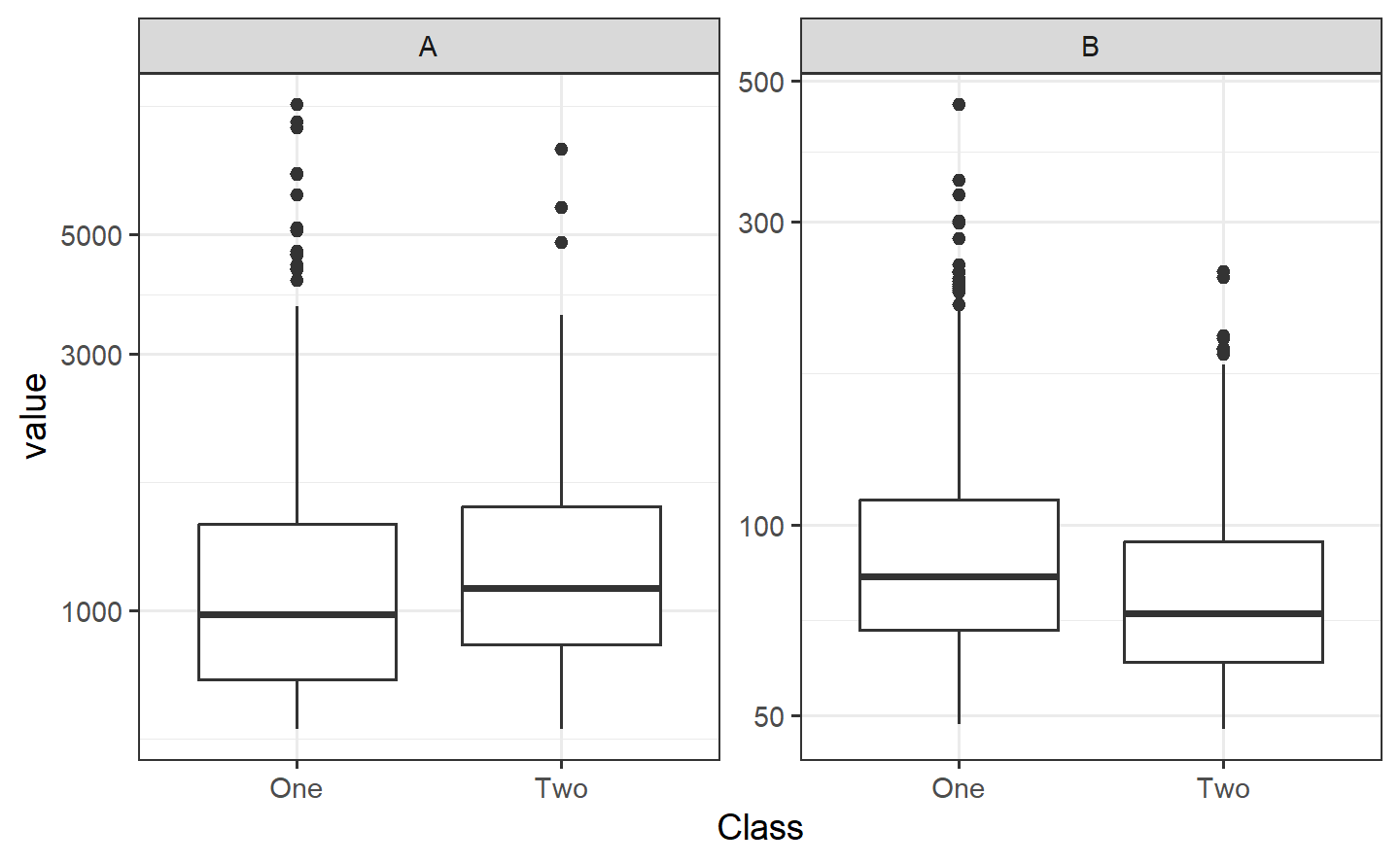

In the first plot above, the separation appears to happen linearly, and a straight, diagonal boundary might do well. We could use glm() directly to create a logistic regression, but we will use the tidymodels infrastructure and start by making a parsnip model object.

logit_mod <- logistic_reg() %>% 
  set_engine("glm")

glm_workflow <-
  workflow() %>%
  add_model(logit_mod)

simple_glm <- 
  glm_workflow %>% 
  add_formula(Class ~ .) %>% 
  fit(data = bivariate_train)
simple_glm
#> ══ Workflow [trained] ══════════════════════════════════════════════════════════
#> Preprocessor: Formula
#> Model: logistic_reg()
#> 
#> ── Preprocessor ────────────────────────────────────────────────────────────────
#> Class ~ .
#> 
#> ── Model ───────────────────────────────────────────────────────────────────────
#> 
#> Call:  stats::glm(formula = ..y ~ ., family = stats::binomial, data = data)
#> 
#> Coefficients:
#> (Intercept)            A            B  
#>    1.731243     0.002622    -0.064411  
#> 
#> Degrees of Freedom: 1008 Total (i.e. Null);  1006 Residual
#> Null Deviance:       1329 
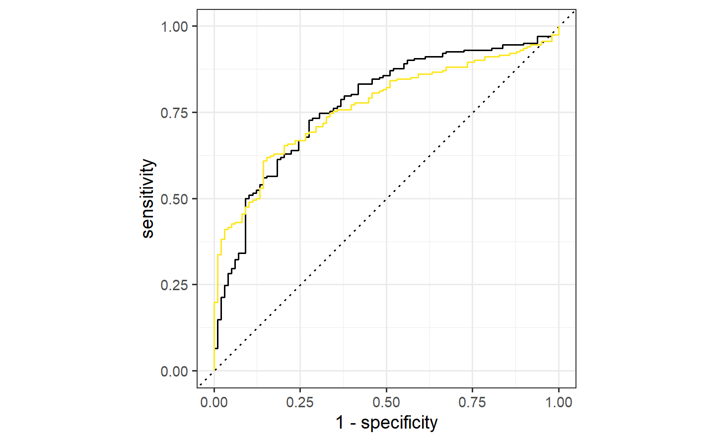
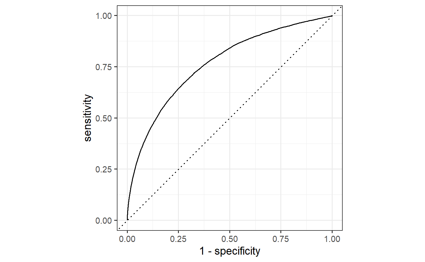
#> Residual Deviance: 1133  AIC: 1139

To evaluate this model, the ROC curve will be computed along with its corresponding AUC.

simple_glm_probs <- 
  predict(simple_glm, bivariate_val, type = "prob") %>% 
  bind_cols(bivariate_val)

simple_glm_roc <- 
  simple_glm_probs %>% 
  roc_curve(Class, .pred_One)

simple_glm_probs %>% roc_auc(Class, .pred_One)
#> # A tibble: 1 × 3
#>   .metric .estimator .estimate
#>   <chr>   <chr>          <dbl>
#> 1 roc_auc binary         0.773

autoplot(simple_glm_roc)

Since there are two correlated predictors with skewed distributions and strictly positive values, it might be intuitive to use their ratio instead of the pair. We’ll try that next by recycling the initial workflow and just adding a different formula:

ratio_glm <- 
  glm_workflow %>% 
  add_formula(Class ~ I(A/B)) %>% 
  fit(data = bivariate_train)

ratio_glm_probs <- 
  predict(ratio_glm, bivariate_val, type = "prob") %>% 
  bind_cols(bivariate_val)

ratio_glm_roc <- 
  ratio_glm_probs %>% 
  roc_curve(Class, .pred_One)

ratio_glm_probs %>% roc_auc(Class, .pred_One)
#> # A tibble: 1 × 3
#>   .metric .estimator .estimate
#>   <chr>   <chr>          <dbl>
#> 1 roc_auc binary         0.765

autoplot(simple_glm_roc) +
  geom_path(
    data = ratio_glm_roc,
    aes(x = 1 - specificity, y = sensitivity),
    col = "#FDE725FF"
  )

More complex feature engineering

Instead of combining the two predictors, would it help the model if we were to resolve the skewness of the variables? To test this theory, one option would be to use the Box-Cox transformation on each predictor individually to see if it recommends a nonlinear transformation. The transformation can encode a variety of different functions including the log transform, square root, inverse, and fractional transformations in-between these.

trans_recipe <- 
  recipe(Class ~ ., data = bivariate_train) %>% 
  step_BoxCox(all_predictors())

trans_glm <- 
  glm_workflow %>% 
  add_recipe(trans_recipe) %>% 
  fit(data = bivariate_train)

trans_glm_probs <- 
  predict(trans_glm, bivariate_val, type = "prob") %>% 
  bind_cols(bivariate_val)

trans_glm_roc <- 
  trans_glm_probs %>% 
  roc_curve(Class, .pred_One)

trans_glm_probs %>% roc_auc(Class, .pred_One)
#> # A tibble: 1 × 3
#>   .metric .estimator .estimate
#>   <chr>   <chr>          <dbl>
#> 1 roc_auc binary         0.815

autoplot(simple_glm_roc) +
  geom_path(
    data = ratio_glm_roc,
    aes(x = 1 - specificity, y = sensitivity),
    col = "#FDE725FF"
  ) +
  geom_path(
    data = trans_glm_roc,
    aes(x = 1 - specificity, y = sensitivity),
    col = "#21908CFF"
  )

ggplot(bivariate_train, aes(1/A, 1/B, col = Class)) + 
  geom_point(alpha = .3) +
  coord_equal(ratio = 1/12)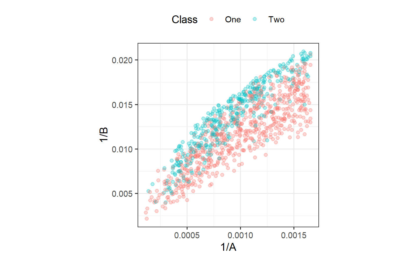

pca_recipe <- 
  trans_recipe %>% 
  step_normalize(A, B) %>% 
  step_pca(A, B, num_comp = 2)

pca_glm <- 
  glm_workflow %>% 
  add_recipe(pca_recipe) %>% 
  fit(data = bivariate_train)

pca_glm_probs <- 
  predict(pca_glm, bivariate_val, type = "prob") %>% 
  bind_cols(bivariate_val)

pac_glm_roc <- 
  pca_glm_probs %>% 
  roc_curve(Class, .pred_One)

pca_glm_probs %>% roc_auc(Class, .pred_One)
#> # A tibble: 1 × 3
#>   .metric .estimator .estimate
#>   <chr>   <chr>          <dbl>
#> 1 roc_auc binary         0.815

# using the test set
test_prob <- 
  predict(trans_glm, bivariate_test, type = "prob") %>% 
  bind_cols(bivariate_test)

test_roc <- 
  test_prob %>% 
  roc_curve(Class, .pred_One)

test_prob %>% roc_auc(Class, .pred_One)
#> # A tibble: 1 × 3
#>   .metric .estimator .estimate
#>   <chr>   <chr>          <dbl>
#> 1 roc_auc binary         0.862

autoplot(test_roc)

1.5 tune

官网：https://tune.tidymodels.org/

1.5.1 Index

The goal of tune is to facilitate hyperparameter tuning for the tidymodels packages. It relies heavily on {recipes}, {parsnip}, and {dials}.

1.5.2 Get started

set.seed(4595)

data_split <- 
  ames %>% 
  mutate(Sale_Price = log10(Sale_Price)) %>% 
  initial_split(strata = Sale_Price)

ames_train <- training(data_split)
ame_test <- testing(data_split)

ames_train %>% 
  select(Sale_Price, Longitude, Latitude) %>% 
  pivot_longer(cols = 2:3,
               names_to = "predictor",
               values_to = "value") %>% 
  ggplot(aes(value, Sale_Price)) +
  geom_point(alpha = .2) +
  geom_smooth(se = FALSE) +
  facet_wrap(~ predictor, scales = "free_x")
#> `geom_smooth()` using method = 'gam' and formula = 'y ~ s(x, bs = "cs")'

ames_rec <- 
  recipe(Sale_Price ~ Gr_Liv_Area + Longitude + Latitude, data = ames_train) %>% 
  step_log(Gr_Liv_Area, base = 10) %>% 
  step_ns(Longitude, deg_free = tune("long df")) %>% 
  step_ns(Latitude, deg_free = tune("lat df"))

The function dials::parameters() can detect and collect the parameters that have been flagged for tuning:

parameters(ames_rec)
#> Warning: `parameters.workflow()` was deprecated in tune 0.1.6.9003.
#> ℹ Please use `hardhat::extract_parameter_set_dials()` instead.
#> Collection of 2 parameters for tuning
#> 
#>  identifier     type    object
#>     long df deg_free nparam[+]
#>      lat df deg_free nparam[+]

The {dials} package has default ranges for many parameters. The generic parameter function for deg_free has a fairly small range:

deg_free()
#> Degrees of Freedom (quantitative)
#> Range: [1, 5]

However, there is a dials function that is more appropriate for splines:

spline_degree()
#> Spline Degrees of Freedom (quantitative)
#> Range: [1, 10]

The parameter objects can be easily changed using the update() function:

ames_param <- 
  ames_rec %>% 
  parameters() %>% 
  update(
    `long df` = spline_degree(),
    `lat df` = spline_degree()
  )

ames_param
#> Collection of 2 parameters for tuning
#> 
#>  identifier     type    object
#>     long df deg_free nparam[+]
#>      lat df deg_free nparam[+]

Grid Search

spline_grid <- grid_max_entropy(ames_param, size = 10)
spline_grid
#> # A tibble: 10 × 2
#>    `long df` `lat df`
#>        <int>    <int>
#>  1         2        4
#>  2         7        7
#>  3         4        6
#>  4        10        4
#>  5         1        8
#>  6         5        1
#>  7         4       10
#>  8         6        4
#>  9        10       10
#> 10         9        1

# A regular grid
df_vals <- seq(2, 18, by = 2)
spline_grid <- expand.grid(`long df` = df_vals,
                           `lat df` = df_vals)

There are two other ingredients that are required before tuning.

First is a model specification. Using {parsnip}, a basic linear model can be used:

# a basic linear model
lm_mod <- linear_reg() %>% set_engine("lm")

# simple 10-fold cross-validation
set.seed(2453)
cv_splits <- vfold_cv(ames_train, v = 10, strata = Sale_Price)

The root mean squared error will be used to measure performance (and this is the default for regression problems).

ames_res <- tune_grid(lm_mod, ames_rec,
                      resamples = cv_splits,
                      grid = spline_grid)
ames_res
#> # Tuning results
#> # 10-fold cross-validation using stratification 
#> # A tibble: 10 × 4
#>    splits             id     .metrics           .notes          
#>    <list>             <chr>  <list>             <list>          
#>  1 <split [1976/221]> Fold01 <tibble [162 × 6]> <tibble [0 × 3]>
#>  2 <split [1976/221]> Fold02 <tibble [162 × 6]> <tibble [0 × 3]>
#>  3 <split [1976/221]> Fold03 <tibble [162 × 6]> <tibble [0 × 3]>
#>  4 <split [1976/221]> Fold04 <tibble [162 × 6]> <tibble [0 × 3]>
#>  5 <split [1977/220]> Fold05 <tibble [162 × 6]> <tibble [0 × 3]>
#>  6 <split [1977/220]> Fold06 <tibble [162 × 6]> <tibble [0 × 3]>
#>  7 <split [1978/219]> Fold07 <tibble [162 × 6]> <tibble [0 × 3]>
#>  8 <split [1978/219]> Fold08 <tibble [162 × 6]> <tibble [0 × 3]>
#>  9 <split [1979/218]> Fold09 <tibble [162 × 6]> <tibble [0 × 3]>
#> 10 <split [1980/217]> Fold10 <tibble [162 × 6]> <tibble [0 × 3]>

The .metrics column has all of the holdout performance estimates for each parameter combination:

ames_res$.metrics[[1]]
#> # A tibble: 162 × 6
#>    `long df` `lat df` .metric .estimator .estimate .config              
#>        <dbl>    <dbl> <chr>   <chr>          <dbl> <chr>                
#>  1         2        2 rmse    standard      0.0985 Preprocessor01_Model1
#>  2         2        2 rsq     standard      0.683  Preprocessor01_Model1
#>  3         4        2 rmse    standard      0.0985 Preprocessor02_Model1
#>  4         4        2 rsq     standard      0.683  Preprocessor02_Model1
#>  5         6        2 rmse    standard      0.0973 Preprocessor03_Model1
#>  6         6        2 rsq     standard      0.690  Preprocessor03_Model1
#>  7         8        2 rmse    standard      0.0962 Preprocessor04_Model1
#>  8         8        2 rsq     standard      0.697  Preprocessor04_Model1
#>  9        10        2 rmse    standard      0.0960 Preprocessor05_Model1
#> 10        10        2 rsq     standard      0.699  Preprocessor05_Model1
#> # ℹ 152 more rows

To get the average metric value for each parameter combination, collect_metrics() can be put to use:

estimates <- collect_metrics(ames_res)
estimates
#> # A tibble: 162 × 8
#>    `long df` `lat df` .metric .estimator   mean     n std_err .config           
#>        <dbl>    <dbl> <chr>   <chr>       <dbl> <int>   <dbl> <chr>             
#>  1         2        2 rmse    standard   0.100     10 0.00145 Preprocessor01_Mo…
#>  2         2        2 rsq     standard   0.674     10 0.00777 Preprocessor01_Mo…
#>  3         4        2 rmse    standard   0.100     10 0.00153 Preprocessor02_Mo…
#>  4         4        2 rsq     standard   0.675     10 0.00814 Preprocessor02_Mo…
#>  5         6        2 rmse    standard   0.0994    10 0.00161 Preprocessor03_Mo…
#>  6         6        2 rsq     standard   0.680     10 0.00885 Preprocessor03_Mo…
#>  7         8        2 rmse    standard   0.0989    10 0.00159 Preprocessor04_Mo…
#>  8         8        2 rsq     standard   0.684     10 0.00946 Preprocessor04_Mo…
#>  9        10        2 rmse    standard   0.0990    10 0.00165 Preprocessor05_Mo…
#> 10        10        2 rsq     standard   0.683     10 0.0101  Preprocessor05_Mo…
#> # ℹ 152 more rows

estimates %>% 
  filter(.metric == "rmse") %>% 
  arrange(mean)
#> # A tibble: 81 × 8
#>    `long df` `lat df` .metric .estimator   mean     n std_err .config           
#>        <dbl>    <dbl> <chr>   <chr>       <dbl> <int>   <dbl> <chr>             
#>  1        16       12 rmse    standard   0.0948    10 0.00120 Preprocessor53_Mo…
#>  2        18       12 rmse    standard   0.0948    10 0.00121 Preprocessor54_Mo…
#>  3        16        8 rmse    standard   0.0949    10 0.00118 Preprocessor35_Mo…
#>  4        16       10 rmse    standard   0.0949    10 0.00118 Preprocessor44_Mo…
#>  5        16       18 rmse    standard   0.0949    10 0.00119 Preprocessor80_Mo…
#>  6        16       16 rmse    standard   0.0949    10 0.00122 Preprocessor71_Mo…
#>  7        18       10 rmse    standard   0.0949    10 0.00119 Preprocessor45_Mo…
#>  8        18        8 rmse    standard   0.0949    10 0.00119 Preprocessor36_Mo…
#>  9        18       18 rmse    standard   0.0950    10 0.00120 Preprocessor81_Mo…
#> 10        16       14 rmse    standard   0.0950    10 0.00117 Preprocessor62_Mo…
#> # ℹ 71 more rows

Smaller degrees of freedom values correspond to more linear functions, but the grid search indicates that more nonlinearity is better. What was the relationship between these two parameters and RMSE?

autoplot(ames_res, metric = "rmse")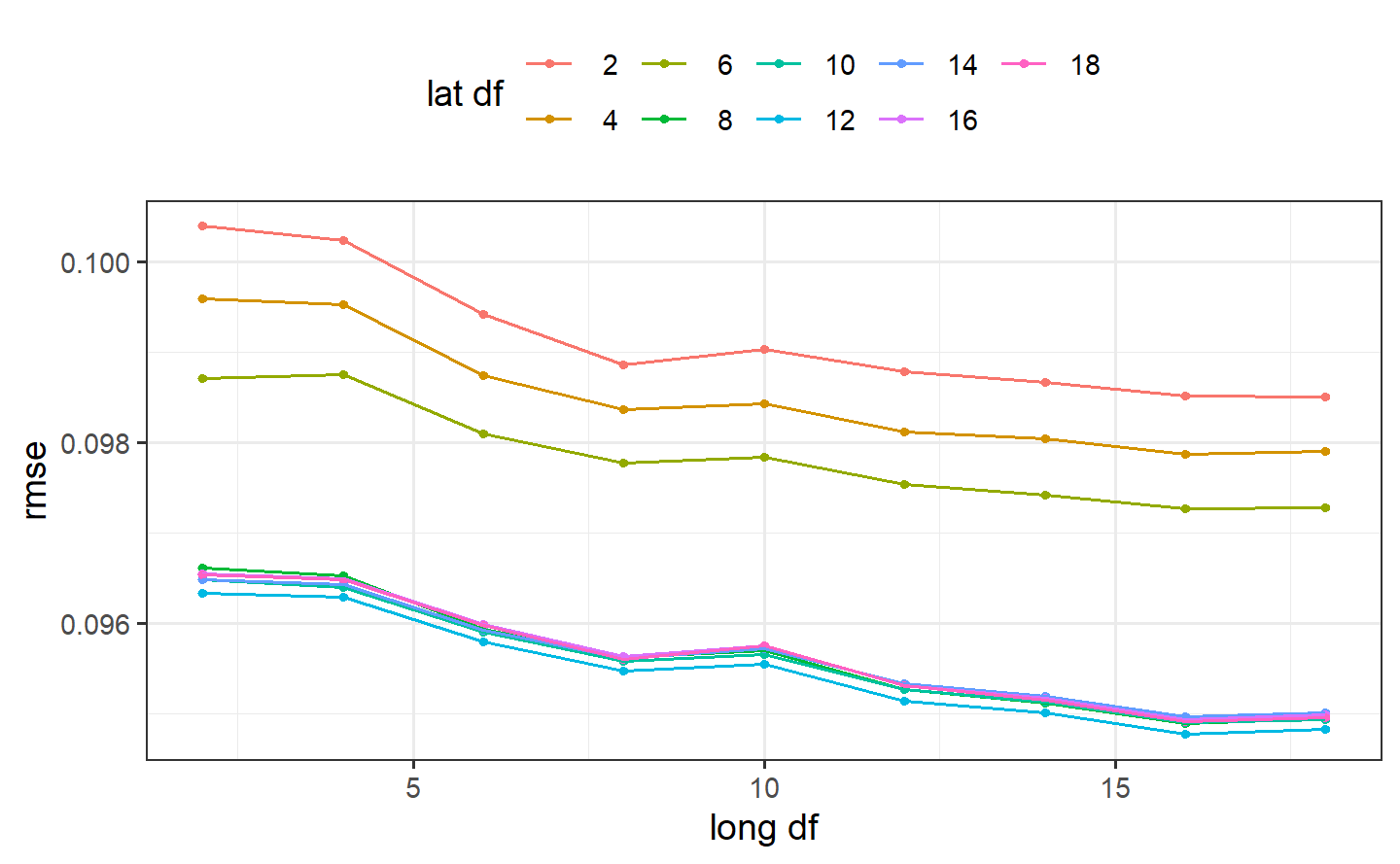

Interestingly, latitude does not do well with degrees of freedom less than 8. How nonlinear are the optimal degrees of freedom?

Let’s plot these spline functions over the data for both good and bad values of deg_free:

ames_train %>% 
  select(Sale_Price, Longitude, Latitude) %>% 
  pivot_longer(cols = 2:3,
               names_to = "predictor",
               values_to = "value") %>% 
  ggplot(aes(value, Sale_Price)) +
  geom_point(alpha = .2) +
  geom_smooth(se = FALSE, method = lm,
              formula = y ~ splines::ns(x, df = 3),
              col = "red") +
  geom_smooth(se = FALSE, method = lm,
              formula = y ~ splines::ns(x, df = 16)) +
  scale_y_log10() +
  facet_wrap(~ predictor, scales = "free_x")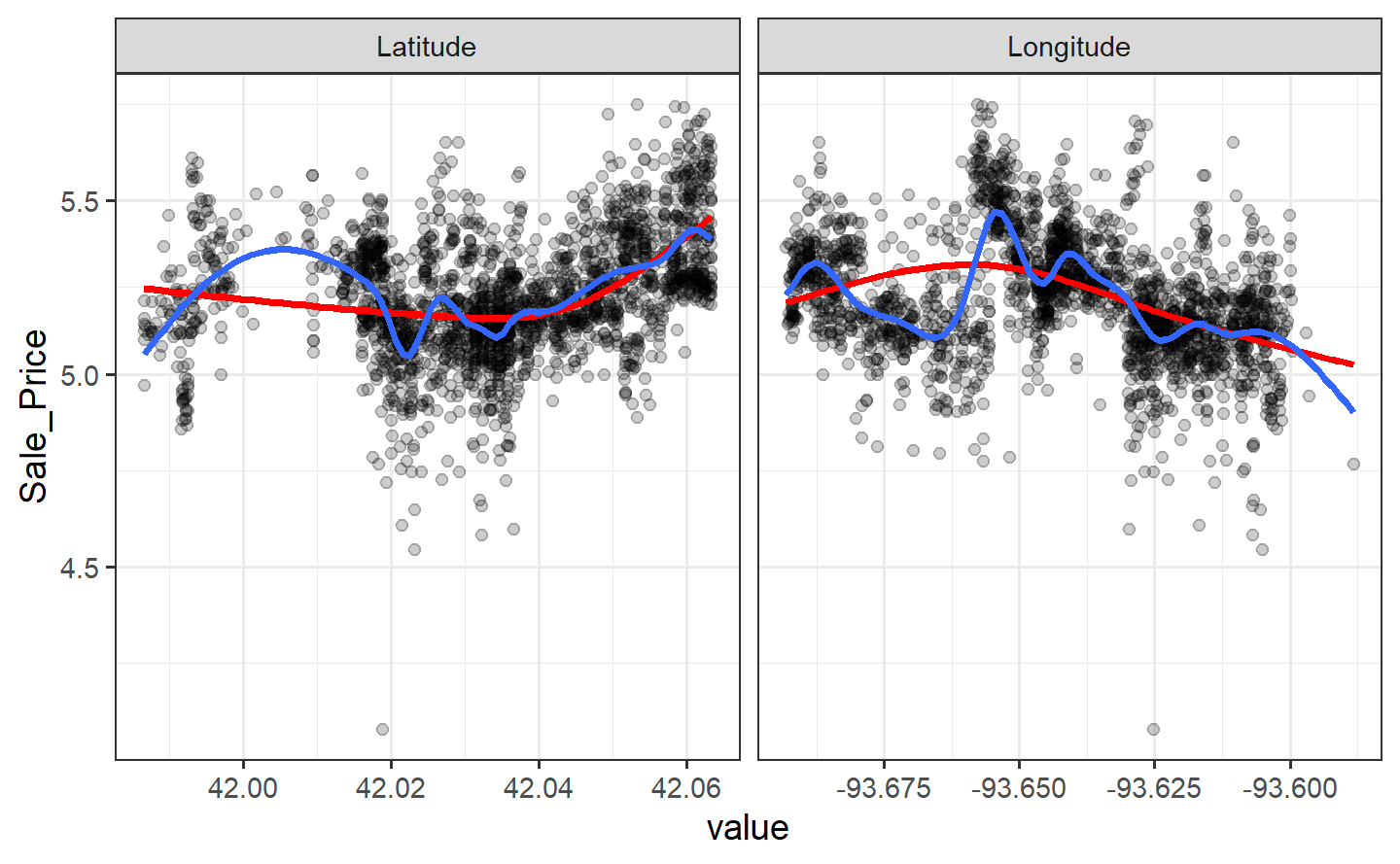

Looking at these plots, the smaller degrees of freedom (red) are clearly under-fitting. Visually, the more complex splines (blue) might indicate that there is overfitting but this would result in poor RMSE values when computed on the hold-out data.

Based on these results, a new recipe would be created with the optimized values (using the entire training set) and this would be combined with a linear model created form the entire training set.

Model Optimization

Instead of a linear regression, a nonlinear model might provide good performance. A K-nearest-neighbor fit will also be optimized. For this example, the number of neighbors and the distance weighting function will be optimized:

knn_mod <- 
  nearest_neighbor(neighbors = tune(), weight_func = tune()) %>% 
  set_engine("kknn") %>% 
  set_mode("regression")

knn_wflow <- 
  workflow() %>% 
  add_model(knn_mod) %>% 
  add_recipe(ames_rec)

knn_param <- 
  knn_wflow %>% 
  parameters() %>% 
  update(
    `long df` = spline_degree(c(2, 18)), 
    `lat df` = spline_degree(c(2, 18)),
    neighbors = neighbors(c(3, 50)),
    weight_func = weight_func(values = c("rectangular", "inv", "gaussian", "triangular"))
  )

# conduct the search
ctrl <- control_bayes(verbose = TRUE)
set.seed(8154)
knn_search <- tune_bayes(knn_wflow, resamples = cv_splits, 
                         initial = 5, iter = 20,
                         param_info = knn_param, control = ctrl)

Visually, the performance gain was:

autoplot(knn_search, type = "performance", metric = "rmse")

The best results here were:

collect_metrics(knn_search) %>% 
  filter(.metric == "rmse") %>% 
  arrange(mean)
#> # A tibble: 18 × 11
#>    neighbors weight_func `long df` `lat df` .metric .estimator   mean     n
#>        <int> <chr>           <int>    <int> <chr>   <chr>       <dbl> <int>
#>  1         7 gaussian           10        8 rmse    standard   0.0826    10
#>  2         9 gaussian            8        8 rmse    standard   0.0829    10
#>  3         9 inv                 8        6 rmse    standard   0.0831    10
#>  4         7 gaussian           11       10 rmse    standard   0.0835    10
#>  5         9 gaussian           11        8 rmse    standard   0.0835    10
#>  6        15 gaussian            4        7 rmse    standard   0.0837    10
#>  7         3 gaussian           10        7 rmse    standard   0.0843    10
#>  8         4 triangular         10        7 rmse    standard   0.0847    10
#>  9         4 inv                 6       10 rmse    standard   0.0853    10
#> 10         5 gaussian           16       13 rmse    standard   0.0857    10
#> 11         7 gaussian           15        3 rmse    standard   0.0869    10
#> 12         5 gaussian           17       17 rmse    standard   0.0879    10
#> 13        30 inv                11        8 rmse    standard   0.0894    10
#> 14        12 inv                18        2 rmse    standard   0.0900    10
#> 15         3 triangular          9       18 rmse    standard   0.0904    10
#> 16        49 triangular          8        4 rmse    standard   0.0914    10
#> 17        34 gaussian           14        9 rmse    standard   0.0926    10
#> 18        19 rectangular         2       16 rmse    standard   0.0981    10
#> # ℹ 3 more variables: std_err <dbl>, .config <chr>, .iter <int>

1.6 yardstick

官网：https://yardstick.tidymodels.org/

1.6.1 Index

{yardstick} is a package to estimate how well models are working using tidy data principles.

head(two_class_example)
#>    truth      Class1       Class2 predicted
#> 1 Class2 0.003589243 0.9964107574    Class2
#> 2 Class1 0.678621054 0.3213789460    Class1
#> 3 Class2 0.110893522 0.8891064779    Class2
#> 4 Class1 0.735161703 0.2648382969    Class1
#> 5 Class2 0.016239960 0.9837600397    Class2
#> 6 Class1 0.999275071 0.0007249286    Class1

metrics(two_class_example, truth, predicted)
#> # A tibble: 2 × 3
#>   .metric  .estimator .estimate
#>   <chr>    <chr>          <dbl>
#> 1 accuracy binary         0.838
#> 2 kap      binary         0.675

two_class_example %>% 
  roc_auc(truth, Class1)
#> # A tibble: 1 × 3
#>   .metric .estimator .estimate
#>   <chr>   <chr>          <dbl>
#> 1 roc_auc binary         0.939

hpc_cv <- hpc_cv %>% as_tibble()
hpc_cv
#> # A tibble: 3,467 × 7
#>    obs   pred     VF      F       M          L Resample
#>    <fct> <fct> <dbl>  <dbl>   <dbl>      <dbl> <chr>   
#>  1 VF    VF    0.914 0.0779 0.00848 0.0000199  Fold01  
#>  2 VF    VF    0.938 0.0571 0.00482 0.0000101  Fold01  
#>  3 VF    VF    0.947 0.0495 0.00316 0.00000500 Fold01  
#>  4 VF    VF    0.929 0.0653 0.00579 0.0000156  Fold01  
#>  5 VF    VF    0.942 0.0543 0.00381 0.00000729 Fold01  
#>  6 VF    VF    0.951 0.0462 0.00272 0.00000384 Fold01  
#>  7 VF    VF    0.914 0.0782 0.00767 0.0000354  Fold01  
#>  8 VF    VF    0.918 0.0744 0.00726 0.0000157  Fold01  
#>  9 VF    VF    0.843 0.128  0.0296  0.000192   Fold01  
#> 10 VF    VF    0.920 0.0728 0.00703 0.0000147  Fold01  
#> # ℹ 3,457 more rows

# Macro averaged multiclass precision
precision(hpc_cv, obs, pred)
#> # A tibble: 1 × 3
#>   .metric   .estimator .estimate
#>   <chr>     <chr>          <dbl>
#> 1 precision macro          0.631

# Micro averaged multiclass precision
precision(hpc_cv, obs, pred, estimator = "micro")
#> # A tibble: 1 × 3
#>   .metric   .estimator .estimate
#>   <chr>     <chr>          <dbl>
#> 1 precision micro          0.709

hpc_cv %>% 
  group_by(Resample) %>% 
  roc_auc(obs, VF:L)
#> # A tibble: 10 × 4
#>    Resample .metric .estimator .estimate
#>    <chr>    <chr>   <chr>          <dbl>
#>  1 Fold01   roc_auc hand_till      0.813
#>  2 Fold02   roc_auc hand_till      0.817
#>  3 Fold03   roc_auc hand_till      0.869
#>  4 Fold04   roc_auc hand_till      0.849
#>  5 Fold05   roc_auc hand_till      0.811
#>  6 Fold06   roc_auc hand_till      0.836
#>  7 Fold07   roc_auc hand_till      0.825
#>  8 Fold08   roc_auc hand_till      0.846
#>  9 Fold09   roc_auc hand_till      0.828
#> 10 Fold10   roc_auc hand_till      0.812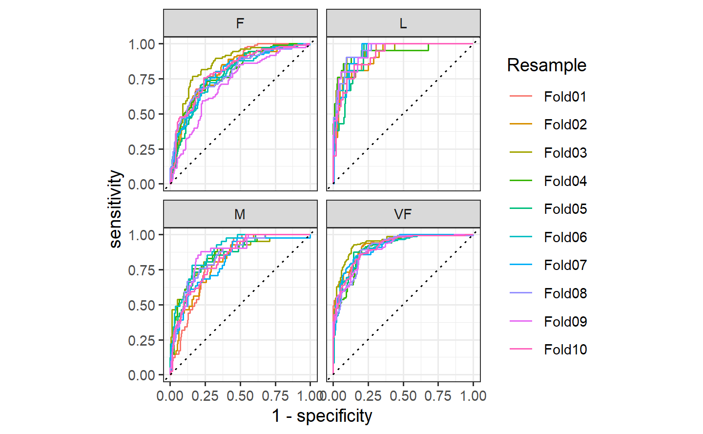

hpc_cv %>% 
  group_by(Resample) %>% 
  roc_curve(obs, VF:L) %>% 
  autoplot()

1.7 broom

官网：https://broom.tidymodels.org/

1.7.1 Index

tidy() produces a tibble() where each row contains information about an important component of the model. For regression models, this often corresponds to regression coefficients. This is can be useful if you want to inspect a model or create custom visualizations.

data("trees")

fit <- lm(Volume ~ Girth + Height, trees)
tidy(fit)
#> # A tibble: 3 × 5
#>   term        estimate std.error statistic  p.value
#>   <chr>          <dbl>     <dbl>     <dbl>    <dbl>
#> 1 (Intercept)  -58.0       8.64      -6.71 2.75e- 7
#> 2 Girth          4.71      0.264     17.8  8.22e-17
#> 3 Height         0.339     0.130      2.61 1.45e- 2

glance() returns a tibble with exactly one row of goodness of fitness measures and related statistics. This is useful to check for model misspecification and to compare many models.

glance(fit)
#> # A tibble: 1 × 12
#>   r.squared adj.r.squared sigma statistic  p.value    df logLik   AIC   BIC
#>       <dbl>         <dbl> <dbl>     <dbl>    <dbl> <dbl>  <dbl> <dbl> <dbl>
#> 1     0.948         0.944  3.88      255. 1.07e-18     2  -84.5  177.  183.
#> # ℹ 3 more variables: deviance <dbl>, df.residual <int>, nobs <int>

augment() adds columns to a dataset, containing information such as fitted values, residuals or cluster assignments. All columns added to a dataset have . prefix to prevent existing columns from being overwritten.

augment(fit, data = trees)
#> # A tibble: 31 × 9
#>    Girth Height Volume .fitted .resid   .hat .sigma   .cooksd .std.resid
#>    <dbl>  <dbl>  <dbl>   <dbl>  <dbl>  <dbl>  <dbl>     <dbl>      <dbl>
#>  1   8.3     70   10.3    4.84  5.46  0.116    3.79 0.0978        1.50  
#>  2   8.6     65   10.3    4.55  5.75  0.147    3.77 0.148         1.60  
#>  3   8.8     63   10.2    4.82  5.38  0.177    3.78 0.167         1.53  
#>  4  10.5     72   16.4   15.9   0.526 0.0592   3.95 0.000409      0.140 
#>  5  10.7     81   18.8   19.9  -1.07  0.121    3.95 0.00394      -0.294 
#>  6  10.8     83   19.7   21.0  -1.32  0.156    3.94 0.00840      -0.370 
#>  7  11       66   15.6   16.2  -0.593 0.115    3.95 0.00114      -0.162 
#>  8  11       75   18.2   19.2  -1.05  0.0515   3.95 0.00138      -0.277 
#>  9  11.1     80   22.6   21.4   1.19  0.0920   3.95 0.00348       0.321 
#> 10  11.2     75   19.9   20.2  -0.288 0.0480   3.95 0.0000968    -0.0759
#> # ℹ 21 more rows

1.8 dials

1.8.1 Index

This package contains infrastructure to create and manage values of tuning parameters for the tidymodels packages.

1.8.2 Get started

In any case, some information is needed to create a grid or to validate whether a candidate value is appropriate (e.g. the number of neighbors should be a positive integer). {dials} is designed to:

• Create an easy to use framework for describing and querying tuning parameters. This can include getting sequences or random tuning values, validating current values, transforming parameters, and other tasks.
• Standardize the names of different parameters. Different packages in R use different argument names for the same quantities. dials proposes some standardized names so that the user doesn’t need to memorize the syntactical minutiae of every package.
• Work with the other tidymodels packages for modeling and machine learning using tidyverse principles.

Numeric Parameters

cost_complexity()
#> Cost-Complexity Parameter (quantitative)
#> Transformer: log-10 [1e-100, Inf]
#> Range (transformed scale): [-10, -1]

Note that this parameter is handled in log units and the default range of values is between 10^-10 and 0.1. The range of possible values can be returned and changed based on some utility functions. We’ll use the pipe operator here:

cost_complexity() %>% range_get()
#> $lower
#> [1] 1e-10
#> 
#> $upper
#> [1] 0.1

cost_complexity() %>% range_set(c(-5, 1))
#> Cost-Complexity Parameter (quantitative)
#> Transformer: log-10 [1e-100, Inf]
#> Range (transformed scale): [-5, 1]

# Or using the `range` argument
cost_complexity(range = c(-5, 1))
#> Cost-Complexity Parameter (quantitative)
#> Transformer: log-10 [1e-100, Inf]
#> Range (transformed scale): [-5, 1]

Values for this parameter can be obtained in a few different ways. To get a sequence of values that span the range:

# Natural units
cost_complexity() %>% value_seq(n = 4)
#> [1] 1e-10 1e-07 1e-04 1e-01

# Stay in the transformed space
cost_complexity() %>% value_seq(n = 4, original = FALSE)
#> [1] -10  -7  -4  -1

Random values can be sampled too:

set.seed(5473)
cost_complexity() %>% value_sample(n = 4)
#> [1] 6.905948e-09 8.463338e-04 3.448626e-06 5.902285e-10

Discrete Parameters

In the discrete case there is no notion of a range. The parameter objects are defined by their discrete values.

weight_func()
#> Distance Weighting Function  (qualitative)
#> 10 possible values include:
#> 'rectangular', 'triangular', 'epanechnikov', 'biweight', 'triweight', 'cos', ...

weight_func() %>% value_set(c("rectangular", "triangular"))
#> Distance Weighting Function  (qualitative)
#> 2 possible values include:
#> 'rectangular' and 'triangular'

weight_func() %>% value_sample(3)
#> [1] "inv"      "biweight" "optimal"

weight_func() %>% value_seq(3)
#> [1] "rectangular"  "triangular"   "epanechnikov"

2 tidymodels get started

地址：https://www.tidymodels.org/start/

2.1 Build a model

library(broom.mixed) # for converting bayesian models to tidy tibbles
library(dotwhisker)  # for visualizing regression results

2.1.1 The sea urchins data

urchins <-
  read_csv("https://tidymodels.org/start/models/urchins.csv", show_col_types = FALSE) %>% 
  setNames(c("food_regime", "initial_volume", "width")) %>% 
  mutate(food_regime = factor(food_regime, levels = c("Initial", "Low", "High")))

urchins
#> # A tibble: 72 × 3
#>    food_regime initial_volume width
#>    <fct>                <dbl> <dbl>
#>  1 Initial                3.5 0.01 
#>  2 Initial                5   0.02 
#>  3 Initial                8   0.061
#>  4 Initial               10   0.051
#>  5 Initial               13   0.041
#>  6 Initial               13   0.061
#>  7 Initial               15   0.041
#>  8 Initial               15   0.071
#>  9 Initial               16   0.092
#> 10 Initial               17   0.051
#> # ℹ 62 more rows

As a first step in modeling, it’s always a good idea to plot the data:

ggplot(urchins, aes(x = initial_volume,
                    y = width,
                    group = food_regime,
                    col = food_regime)) +
  geom_point() +
  geom_smooth(method = lm, se = FALSE) +
  scale_color_viridis_d(option = "plasma", end = .7)
#> `geom_smooth()` using formula = 'y ~ x'

We can see that urchins that were larger in volume at the start of the experiment tended to have wider sutures at the end, but the slopes of the lines look different so this effect may depend on the feeding regime condition.

2.1.2 Build and fit a model

lm_fit <- linear_reg() %>% 
  fit(width ~ initial_volume * food_regime, data = urchins)
lm_fit
#> parsnip model object
#> 
#> 
#> Call:
#> stats::lm(formula = width ~ initial_volume * food_regime, data = data)
#> 
#> Coefficients:
#>                    (Intercept)                  initial_volume  
#>                      0.0331216                       0.0015546  
#>                 food_regimeLow                 food_regimeHigh  
#>                      0.0197824                       0.0214111  
#>  initial_volume:food_regimeLow  initial_volume:food_regimeHigh  
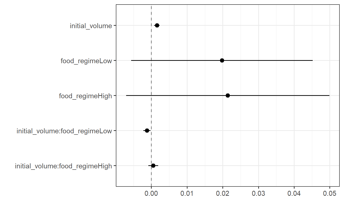
#>                     -0.0012594                       0.0005254

tidy(lm_fit)
#> # A tibble: 6 × 5
#>   term                            estimate std.error statistic  p.value
#>   <chr>                              <dbl>     <dbl>     <dbl>    <dbl>
#> 1 (Intercept)                     0.0331    0.00962      3.44  0.00100 
#> 2 initial_volume                  0.00155   0.000398     3.91  0.000222
#> 3 food_regimeLow                  0.0198    0.0130       1.52  0.133   
#> 4 food_regimeHigh                 0.0214    0.0145       1.47  0.145   
#> 5 initial_volume:food_regimeLow  -0.00126   0.000510    -2.47  0.0162  
#> 6 initial_volume:food_regimeHigh  0.000525  0.000702     0.748 0.457

This kind of output can be used to generate a dot-and-whisker plot of our regression results using the {dotwhisker} package:

tidy(lm_fit) %>% 
  dwplot(dot_args = list(size = 2, color = "black"),
         whisker_args = list(color = "black"),
         vline = geom_vline(xintercept = 0, color = "grey50",
                            linetype = 2))

2.1.3 Use a model to predict

new_points <- expand_grid(initial_volume = 20,
                          food_regime = c("Initial", "Low", "High"))
new_points
#> # A tibble: 3 × 2
#>   initial_volume food_regime
#>            <dbl> <chr>      
#> 1             20 Initial    
#> 2             20 Low        
#> 3             20 High

mean_pred <- predict(lm_fit, new_data = new_points)
mean_pred
#> # A tibble: 3 × 1
#>    .pred
#>    <dbl>
#> 1 0.0642
#> 2 0.0588
#> 3 0.0961

conf_int_pred <- predict(lm_fit, new_data = new_points, type = "conf_int")
conf_int_pred
#> # A tibble: 3 × 2
#>   .pred_lower .pred_upper
#>         <dbl>       <dbl>
#> 1      0.0555      0.0729
#> 2      0.0499      0.0678
#> 3      0.0870      0.105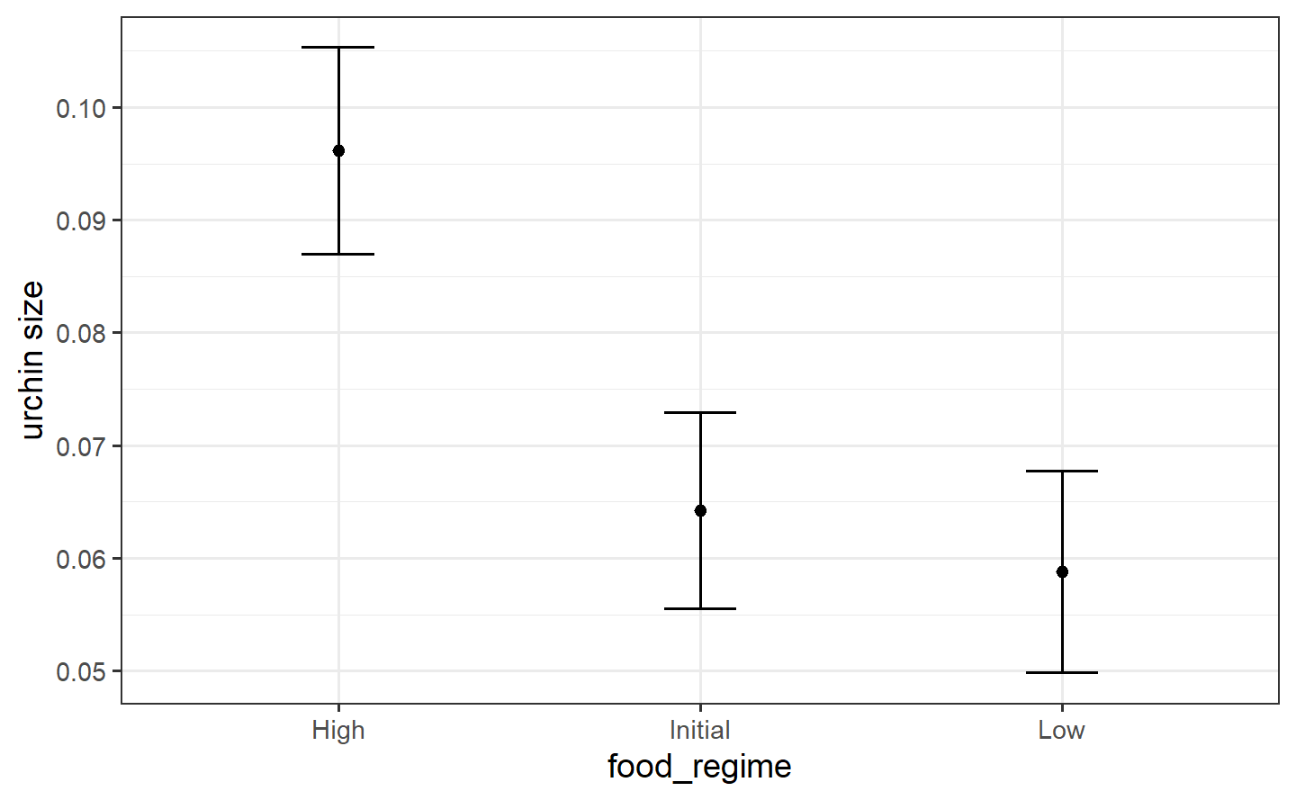

new_points %>% 
  bind_cols(mean_pred) %>% 
  bind_cols(conf_int_pred) %>% 
  ggplot(aes(x = food_regime)) +
  geom_point(aes(y = .pred)) + 
  geom_errorbar(aes(ymin = .pred_lower,
                    ymax = .pred_upper),
                width = .2) +
  labs(y = "urchin size")

2.1.4 Model with a different engine

# set the prior distribution
prior_dist <- rstanarm::student_t(df = 1)

set.seed(123)

# make the paarsnip model
bayes_mod <- linear_reg() %>% 
  set_engine("stan",
             prior_intercept = prior_dist,
             prior = prior_dist)

# train the model
bayes_fit <- 
  bayes_mod %>% 
  fit(width ~ initial_volume * food_regime, data = urchins)

print(bayes_fit, digits = 5)
#> parsnip model object
#> 
#> stan_glm
#>  family:       gaussian [identity]
#>  formula:      width ~ initial_volume * food_regime
#>  observations: 72
#>  predictors:   6
#> ------
#>                                Median   MAD_SD  
#> (Intercept)                     0.03330  0.00933
#> initial_volume                  0.00155  0.00039
#> food_regimeLow                  0.01963  0.01278
#> food_regimeHigh                 0.02089  0.01454
#> initial_volume:food_regimeLow  -0.00126  0.00051
#> initial_volume:food_regimeHigh  0.00055  0.00072
#> 
#> Auxiliary parameter(s):
#>       Median  MAD_SD 
#> sigma 0.02128 0.00186
#> 
#> ------
#> * For help interpreting the printed output see ?print.stanreg
#> * For info on the priors used see ?prior_summary.stanreg

tidy(bayes_fit, conf.int = TRUE)
#> # A tibble: 6 × 5
#>   term                            estimate std.error  conf.low conf.high
#>   <chr>                              <dbl>     <dbl>     <dbl>     <dbl>
#> 1 (Intercept)                     0.0333    0.00933   0.0177    0.0486  
#> 2 initial_volume                  0.00155   0.000395  0.000882  0.00220 
#> 3 food_regimeLow                  0.0196    0.0128   -0.00190   0.0408  
#> 4 food_regimeHigh                 0.0209    0.0145   -0.00296   0.0456  
#> 5 initial_volume:food_regimeLow  -0.00126   0.000515 -0.00208  -0.000411
#> 6 initial_volume:food_regimeHigh  0.000550  0.000717 -0.000643  0.00168

2.2 Preprocess your data with recipes

library(tidymodels)
library(tidyverse)

library(nycflights13)    # for flight data
library(skimr)           # for variable summaries

Let’s use the nycflights13 data to predict whether a plane arrives more than 30 minutes late.

flight_data <- flights %>% 
  mutate(
    arr_delay = factor(ifelse(arr_delay >= 30, "late", "on_time")),
    date = as_date(time_hour)
  ) %>% 
  inner_join(weather, join_by(origin, time_hour)) %>% 
  select(dep_time, flight, origin, dest, air_time, distance, 
         carrier, date, arr_delay, time_hour) %>% 
  drop_na() %>% 
  # For creating models, it is better to have qualitative columns
  # encoded as factors (instead of character strings)
  mutate(across(where(is.character), as_factor))

flight_data %>% 
  count(arr_delay) %>% 
  mutate(prop = n / sum(n))
#> # A tibble: 2 × 3
#>   arr_delay      n  prop
#>   <fct>      <int> <dbl>
#> 1 late       52540 0.161
#> 2 on_time   273279 0.839

We can see that about 16% of the flights in this data set arrived more than 30 minutes late.

glimpse(flight_data)
#> Rows: 325,819
#> Columns: 10
#> $ dep_time  <int> 517, 533, 542, 544, 554, 554, 555, 557, 557, 558, 558, 558, …
#> $ flight    <int> 1545, 1714, 1141, 725, 461, 1696, 507, 5708, 79, 301, 49, 71…
#> $ origin    <fct> EWR, LGA, JFK, JFK, LGA, EWR, EWR, LGA, JFK, LGA, JFK, JFK, …
#> $ dest      <fct> IAH, IAH, MIA, BQN, ATL, ORD, FLL, IAD, MCO, ORD, PBI, TPA, …
#> $ air_time  <dbl> 227, 227, 160, 183, 116, 150, 158, 53, 140, 138, 149, 158, 3…
#> $ distance  <dbl> 1400, 1416, 1089, 1576, 762, 719, 1065, 229, 944, 733, 1028,…
#> $ carrier   <fct> UA, UA, AA, B6, DL, UA, B6, EV, B6, AA, B6, B6, UA, UA, AA, …
#> $ date      <date> 2013-01-01, 2013-01-01, 2013-01-01, 2013-01-01, 2013-01-01,…
#> $ arr_delay <fct> on_time, on_time, late, on_time, on_time, on_time, on_time, …
#> $ time_hour <dttm> 2013-01-01 05:00:00, 2013-01-01 05:00:00, 2013-01-01 05:00:…

flight_data %>% skim(dest, carrier)

Data summary

Name	Piped data
Number of rows	325819
Number of columns	10
_______________________
Column type frequency:
factor	2
________________________
Group variables	None

Variable type: factor

skim_variable	n_missing	complete_rate	ordered	n_unique	top_counts
dest	0	1	FALSE	104	ATL: 16771, ORD: 16507, LAX: 15942, BOS: 14948
carrier	0	1	FALSE	16	UA: 57489, B6: 53715, EV: 50868, DL: 47465

Because we’ll be using a simple logistic regression model, the variables dest and carrier will be converted to dummy variables. However, some of these values do not occur very frequently and this could complicate our analysis. We’ll discuss specific steps later in this article that we can add to our recipe to address this issue before modeling.

2.2.1 Data splitting

set.seed(222)

data_split <- initial_split(flight_data, prop = 3/4)

train_data <- training(data_split)
test_data <- testing(data_split)

2.2.2 Create recipe and roles

We can use the update_role() function to let recipes know that flight and time_hour are variables with a custom role that we called "ID" (a role can have any character value). Whereas our formula included all variables in the training set other than arr_delay as predictors, this tells the recipe to keep these two variables but not use them as either outcomes or predictors.

flights_rec <- 
  recipe(arr_delay ~ ., data = train_data) %>% 
  update_role(flight, time_hour, new_role = "ID")

To get the current set of variables and roles, use the summary() function:

summary(flights_rec)
#> # A tibble: 10 × 4
#>    variable  type      role      source  
#>    <chr>     <list>    <chr>     <chr>   
#>  1 dep_time  <chr [2]> predictor original
#>  2 flight    <chr [2]> ID        original
#>  3 origin    <chr [3]> predictor original
#>  4 dest      <chr [3]> predictor original
#>  5 air_time  <chr [2]> predictor original
#>  6 distance  <chr [2]> predictor original
#>  7 carrier   <chr [3]> predictor original
#>  8 date      <chr [1]> predictor original
#>  9 time_hour <chr [1]> ID        original
#> 10 arr_delay <chr [3]> outcome   original

2.2.3 Create features

It’s possible that the numeric date variable is a good option for modeling; perhaps the model would benefit from a linear trend between the log-odds of a late arrival and the numeric date variable. However, it might be better to add model terms derived from the date that have a better potential to be important to the model. For example, we could derive the following meaningful features from the single date variable:

• the day of the week,
• the month, and
• whether or not the date corresponds to a holiday.

Let’s do all three of these by adding steps to our recipe:

flights_rec <- 
  recipe(arr_delay ~ ., data = train_data) %>% 
  update_role(flight, time_hour, new_role = "ID") %>% 
  step_date(date, features = c("dow", "month")) %>% 
  step_holiday(date,
               holidays = timeDate::listHolidays("US"),
               keep_original_cols = FALSE)

Unlike the standard model formula methods in R, a recipe does not automatically create these dummy variables for you; you’ll need to tell your recipe to add this step. This is for two reasons. First, many models do not require numeric predictors, so dummy variables may not always be preferred. Second, recipes can also be used for purposes outside of modeling, where non-dummy versions of the variables may work better. For example, you may want to make a table or a plot with a variable as a single factor. For those reasons, you need to explicitly tell recipes to create dummy variables using step_dummy():

flights_rec <- 
  recipe(arr_delay ~ ., data = train_data) %>% 
  update_role(flight, time_hour, new_role = "ID") %>% 
  step_date(date, features = c("dow", "month")) %>%               
  step_holiday(date, 
               holidays = timeDate::listHolidays("US"), 
               keep_original_cols = FALSE) %>%
  step_dummy(all_nominal_predictors())

We need one final step to add to our recipe. Since carrier and dest have some infrequently occurring factor values, it is possible that dummy variables might be created for values that don’t exist in the training set. For example, there is one destination that is only in the test set:

test_data %>% 
  distinct(dest) %>% 
  anti_join(train_data, join_by(dest))
#> # A tibble: 1 × 1
#>   dest 
#>   <fct>
#> 1 LEX

When the recipe is applied to the training set, a column is made for LEX because the factor levels come from flight_data (not the training set), but this column will contain all zeros. This is a “zero-variance predictor” that has no information within the column. While some R functions will not produce an error for such predictors, it usually causes warnings and other issues. step_zv() will remove columns from the data when the training set data have a single value, so it is added to the recipe after step_dummy():

flights_rec <- 
  recipe(arr_delay ~ ., data = train_data) %>% 
  update_role(flight, time_hour, new_role = "ID") %>% 
  step_date(date, features = c("dow", "month")) %>%
  step_holiday(date, 
               holidays = timeDate::listHolidays("US"), 
               keep_original_cols = FALSE) %>% 
  step_dummy(all_nominal_predictors()) %>%
  step_zv(all_predictors())

2.2.4 Fit a model with a recipe

lr_mod <- 
  logistic_reg() %>% 
  set_engine("glm")

We will want to use our recipe across several steps as we train and test our model. We will:

• Process the recipe using the training set: This involves any estimation or calculations based on the training set. For our recipe, the training set will be used to determine which predictors should be converted to dummy variables and which predictors will have zero-variance in the training set, and should be slated for removal.

• Apply the recipe to the training set: We create the final predictor set on the training set.

• Apply the recipe to the test set: We create the final predictor set on the test set. Nothing is recomputed and no information from the test set is used here; the dummy variable and zero-variance results from the training set are applied to the test set.

To simplify this process, we can use a model workflow, which pairs a model and recipe together. This is a straightforward approach because different recipes are often needed for different models, so when a model and recipe are bundled, it becomes easier to train and test workflows. We’ll use the workflows package from tidymodels to bundle our parsnip model (lr_mod) with our recipe (flights_rec).

flights_wflow <- 
  workflow() %>% 
  add_model(lr_mod) %>% 
  add_recipe(flights_rec)

flights_wflow
#> ══ Workflow ════════════════════════════════════════════════════════════════════
#> Preprocessor: Recipe
#> Model: logistic_reg()
#> 
#> ── Preprocessor ────────────────────────────────────────────────────────────────
#> 4 Recipe Steps
#> 
#> • step_date()
#> • step_holiday()
#> • step_dummy()
#> • step_zv()
#> 
#> ── Model ───────────────────────────────────────────────────────────────────────
#> Logistic Regression Model Specification (classification)
#> 
#> Computational engine: glm

Now, there is a single function that can be used to prepare the recipe and train the model from the resulting predictors:

flights_fit <- 
  flights_wflow %>% 
  fit(data = train_data)

This object has the finalized recipe and fitted model objects inside. You may want to extract the model or recipe objects from the workflow. To do this, you can use the helper functions extract_fit_parsnip() and extract_recipe(). For example, here we pull the fitted model object then use the broom::tidy() function to get a tidy tibble of model coefficients:

flights_fit %>% 
  extract_fit_parsnip() %>% 
  tidy()
#> # A tibble: 158 × 5
#>    term                         estimate std.error statistic  p.value
#>    <chr>                           <dbl>     <dbl>     <dbl>    <dbl>
#>  1 (Intercept)                   6.56    2.10           3.12 1.80e- 3
#>  2 dep_time                     -0.00166 0.0000141   -118.   0       
#>  3 air_time                     -0.0440  0.000563     -78.2  0       
#>  4 distance                      0.00508 0.00150        3.38 7.13e- 4
#>  5 date_USChristmasDay           1.35    0.178          7.59 3.32e-14
#>  6 date_USColumbusDay            0.721   0.170          4.23 2.33e- 5
#>  7 date_USCPulaskisBirthday      0.804   0.139          5.78 7.38e- 9
#>  8 date_USDecorationMemorialDay  0.582   0.117          4.96 7.22e- 7
#>  9 date_USElectionDay            0.945   0.190          4.97 6.73e- 7
#> 10 date_USGoodFriday             1.24    0.167          7.44 1.04e-13
#> # ℹ 148 more rows

2.2.5 Use a trained workflow to predict

Our goal was to predict whether a plane arrives more than 30 minutes late. We have just:

• Built the model (lr_mod),

• Created a preprocessing recipe (flights_rec),

• Bundled the model and recipe (flights_wflow), and

• Trained our workflow using a single call to fit().

The next step is to use the trained workflow (flights_fit) to predict with the unseen test data, which we will do with a single call to predict(). The predict() method applies the recipe to the new data, then passes them to the fitted model.

predict(flights_fit, test_data)
#> # A tibble: 81,455 × 1
#>    .pred_class
#>    <fct>      
#>  1 on_time    
#>  2 on_time    
#>  3 on_time    
#>  4 on_time    
#>  5 on_time    
#>  6 on_time    
#>  7 on_time    
#>  8 on_time    
#>  9 on_time    
#> 10 on_time    
#> # ℹ 81,445 more rows

Because our outcome variable here is a factor, the output from predict() returns the predicted class: late versus on_time. But, let’s say we want the predicted class probabilities for each flight instead. To return those, we can specify type = "prob" when we use predict() or use augment() with the model plus test data to save them together:

flights_aug <- 
  augment(flights_fit, test_data)

flights_aug %>% 
  select(arr_delay, time_hour, flight,
         .pred_class, .pred_on_time)
#> # A tibble: 81,455 × 5
#>    arr_delay time_hour           flight .pred_class .pred_on_time
#>    <fct>     <dttm>               <int> <fct>               <dbl>
#>  1 on_time   2013-01-01 05:00:00   1545 on_time             0.945
#>  2 on_time   2013-01-01 05:00:00   1714 on_time             0.949
#>  3 on_time   2013-01-01 06:00:00    507 on_time             0.964
#>  4 on_time   2013-01-01 06:00:00   5708 on_time             0.961
#>  5 on_time   2013-01-01 06:00:00     71 on_time             0.962
#>  6 on_time   2013-01-01 06:00:00    194 on_time             0.975
#>  7 on_time   2013-01-01 06:00:00   1124 on_time             0.963
#>  8 on_time   2013-01-01 05:00:00   1806 on_time             0.981
#>  9 on_time   2013-01-01 06:00:00   1187 on_time             0.935
#> 10 on_time   2013-01-01 06:00:00   4650 on_time             0.931
#> # ℹ 81,445 more rows

Let’s use the area under the ROC curve as our metric, computed using roc_curve() and roc_auc() from the yardstick package.

flights_aug %>% 
  roc_curve(truth = arr_delay, .pred_late) %>% 
  autoplot()

Similarly, roc_auc() estimates the area under the curve:

flights_aug %>% 
  roc_auc(truth = arr_delay, .pred_late)
#> # A tibble: 1 × 3
#>   .metric .estimator .estimate
#>   <chr>   <chr>          <dbl>
#> 1 roc_auc binary         0.764

2.3 Evaluate your model with resampling

library(modeldata)

2.3.1 The cell image data

data(cells)
cells
#> # A tibble: 2,019 × 58
#>    case  class angle_ch_1 area_ch_1 avg_inten_ch_1 avg_inten_ch_2 avg_inten_ch_3
#>    <fct> <fct>      <dbl>     <int>          <dbl>          <dbl>          <dbl>
#>  1 Test  PS        143.         185           15.7           4.95           9.55
#>  2 Train PS        134.         819           31.9         207.            69.9 
#>  3 Train WS        107.         431           28.0         116.            63.9 
#>  4 Train PS         69.2        298           19.5         102.            28.2 
#>  5 Test  PS          2.89       285           24.3         112.            20.5 
#>  6 Test  WS         40.7        172          326.          654.           129.  
#>  7 Test  WS        174.         177          260.          596.           124.  
#>  8 Test  PS        180.         251           18.3           5.73          17.2 
#>  9 Test  WS         18.9        495           16.1          89.5           13.7 
#> 10 Test  WS        153.         384           17.7          89.9           20.4 
#> # ℹ 2,009 more rows
#> # ℹ 51 more variables: avg_inten_ch_4 <dbl>, convex_hull_area_ratio_ch_1 <dbl>,
#> #   convex_hull_perim_ratio_ch_1 <dbl>, diff_inten_density_ch_1 <dbl>,
#> #   diff_inten_density_ch_3 <dbl>, diff_inten_density_ch_4 <dbl>,
#> #   entropy_inten_ch_1 <dbl>, entropy_inten_ch_3 <dbl>,
#> #   entropy_inten_ch_4 <dbl>, eq_circ_diam_ch_1 <dbl>,
#> #   eq_ellipse_lwr_ch_1 <dbl>, eq_ellipse_oblate_vol_ch_1 <dbl>, …

2.3.2 Predicting image segmentation quality

A cell-based experiment might involve millions of cells so it is unfeasible to visually assess them all. Instead, a subsample can be created and these cells can be manually labeled by experts as either poorly segmented (PS) or well-segmented (WS). If we can predict these labels accurately, the larger data set can be improved by filtering out the cells most likely to be poorly segmented.

2.3.3 Back to the cells data

The rates of the classes are somewhat imbalanced; there are more poorly segmented cells than well-segmented cells:

cells %>% 
  count(class) %>% 
  mutate(prop = n / sum(n))
#> # A tibble: 2 × 3
#>   class     n  prop
#>   <fct> <int> <dbl>
#> 1 PS     1300 0.644
#> 2 WS      719 0.356

2.3.4 Data splitting

set.seed(123)
cell_split <- initial_split(cells %>% select(-case),
                            strata = class)

Here we used the strata argument, which conducts a stratified split. This ensures that, despite the imbalance we noticed in our class variable, our training and test data sets will keep roughly the same proportions of poorly and well-segmented cells as in the original data. After the initial_split, the training() and testing() functions return the actual data sets.

cell_train <- training(cell_split)
cell_test <- testing(cell_split)

# training set proportions by class
cell_train %>% 
  count(class) %>% 
  mutate(prop = n / sum(n))
#> # A tibble: 2 × 3
#>   class     n  prop
#>   <fct> <int> <dbl>
#> 1 PS      975 0.644
#> 2 WS      539 0.356

# test set proportions by class
cell_test %>% 
  count(class) %>% 
  mutate(prop =  n / sum(n))
#> # A tibble: 2 × 3
#>   class     n  prop
#>   <fct> <int> <dbl>
#> 1 PS      325 0.644
#> 2 WS      180 0.356

2.3.5 Modeling

One of the benefits of a random forest model is that it is very low maintenance; it requires very little preprocessing of the data and the default parameters tend to give reasonable results. For that reason, we won’t create a recipe for the cells data.

To fit a random forest model on the training set, let’s use the {parsnip} package with the {ranger} engine. We first define the model that we want to create:

rf_mod <- 
  rand_forest(trees = 1000) %>% 
  set_engine("ranger") %>% 
  set_mode("classification")

set.seed(234)

rf_fit <- 
  rf_mod %>% 
  fit(class ~ ., data = cell_train)

rf_fit
#> parsnip model object
#> 
#> Ranger result
#> 
#> Call:
#>  ranger::ranger(x = maybe_data_frame(x), y = y, num.trees = ~1000,      num.threads = 1, verbose = FALSE, seed = sample.int(10^5,          1), probability = TRUE) 
#> 
#> Type:                             Probability estimation 
#> Number of trees:                  1000 
#> Sample size:                      1514 
#> Number of independent variables:  56 
#> Mtry:                             7 
#> Target node size:                 10 
#> Variable importance mode:         none 
#> Splitrule:                        gini 
#> OOB prediction error (Brier s.):  0.1187479

2.3.6 Estimating performance

rf_testing_pred <- 
  predict(rf_fit, cell_test) %>% 
  bind_cols(predict(rf_fit, cell_test, type = "prob")) %>% 
  bind_cols(cell_test %>% select(class))

rf_testing_pred %>% 
  roc_auc(truth = class, .pred_PS)
#> # A tibble: 1 × 3
#>   .metric .estimator .estimate
#>   <chr>   <chr>          <dbl>
#> 1 roc_auc binary         0.891

rf_testing_pred %>% 
  accuracy(truth = class, .pred_class)
#> # A tibble: 1 × 3
#>   .metric  .estimator .estimate
#>   <chr>    <chr>          <dbl>
#> 1 accuracy binary         0.814

2.3.7 Resampling to the rescue

The final resampling estimates for the model are the averages of the performance statistics replicates.

2.3.8 Fit a model with resampling

set.seed(345)

folds <- vfold_cv(cell_train, v = 10)
folds
#> #  10-fold cross-validation 
#> # A tibble: 10 × 2
#>    splits             id    
#>    <list>             <chr> 
#>  1 <split [1362/152]> Fold01
#>  2 <split [1362/152]> Fold02
#>  3 <split [1362/152]> Fold03
#>  4 <split [1362/152]> Fold04
#>  5 <split [1363/151]> Fold05
#>  6 <split [1363/151]> Fold06
#>  7 <split [1363/151]> Fold07
#>  8 <split [1363/151]> Fold08
#>  9 <split [1363/151]> Fold09
#> 10 <split [1363/151]> Fold10

The list column for splits contains the information on which rows belong in the analysis and assessment sets. There are functions that can be used to extract the individual resampled data called analysis() and assessment().

You have several options for building an object for resampling:

• Resample a model specification preprocessed with a formula or recipe, or
• Resample a workflow() that bundles together a model specification and formula/recipe.

For this example, let’s use a workflow() that bundles together the random forest model and a formula, since we are not using a recipe. Whichever of these options you use, the syntax to fit_resamples() is very similar to fit():

rf_wf <- 
  workflow() %>% 
  add_model(rf_mod) %>% 
  add_formula(class ~ .)

set.seed(456)
rf_fit_rs <- 
  rf_wf %>% 
  fit_resamples(folds)

rf_fit_rs
#> # Resampling results
#> # 10-fold cross-validation 
#> # A tibble: 10 × 4
#>    splits             id     .metrics         .notes          
#>    <list>             <chr>  <list>           <list>          
#>  1 <split [1362/152]> Fold01 <tibble [2 × 4]> <tibble [0 × 3]>
#>  2 <split [1362/152]> Fold02 <tibble [2 × 4]> <tibble [0 × 3]>
#>  3 <split [1362/152]> Fold03 <tibble [2 × 4]> <tibble [0 × 3]>
#>  4 <split [1362/152]> Fold04 <tibble [2 × 4]> <tibble [0 × 3]>
#>  5 <split [1363/151]> Fold05 <tibble [2 × 4]> <tibble [0 × 3]>
#>  6 <split [1363/151]> Fold06 <tibble [2 × 4]> <tibble [0 × 3]>
#>  7 <split [1363/151]> Fold07 <tibble [2 × 4]> <tibble [0 × 3]>
#>  8 <split [1363/151]> Fold08 <tibble [2 × 4]> <tibble [0 × 3]>
#>  9 <split [1363/151]> Fold09 <tibble [2 × 4]> <tibble [0 × 3]>
#> 10 <split [1363/151]> Fold10 <tibble [2 × 4]> <tibble [0 × 3]>

The results are similar to the folds results with some extra columns. The column .metrics contains the performance statistics created from the 10 assessment sets. These can be manually unnested but the tune package contains a number of simple functions that can extract these data:

collect_metrics(rf_fit_rs)
#> # A tibble: 2 × 6
#>   .metric  .estimator  mean     n std_err .config             
#>   <chr>    <chr>      <dbl> <int>   <dbl> <chr>               
#> 1 accuracy binary     0.833    10 0.00876 Preprocessor1_Model1
#> 2 roc_auc  binary     0.905    10 0.00627 Preprocessor1_Model1

Think about these values we now have for accuracy and AUC. These performance metrics are now more realistic (i.e. lower) than our ill-advised first attempt at computing performance metrics in the section above. If we wanted to try different model types for this data set, we could more confidently compare performance metrics computed using resampling to choose between models. Also, remember that at the end of our project, we return to our test set to estimate final model performance.

Resampling allows us to simulate how well our model will perform on new data, and the test set acts as the final, unbiased check for our model’s performance.

2.4 Tune model parameters

2.4.1 Introduction

Some model parameters cannot be learned directly from a data set during model training; these kinds of parameters are called hyperparameters. Some examples of hyperparameters include the number of predictors that are sampled at splits in a tree-based model (we call this mtry in tidymodels) or the learning rate in a boosted tree model (we call this learn_rate). Instead of learning these kinds of hyperparameters during model training, we can estimate the best values for these values by training many models on resampled data sets and exploring how well all these models perform. This process is called tuning.

library(rpart.plot)
library(vip)

2.4.2 Predicting image segemention, but better

Random forest models are a tree-based ensemble method, and typically perform well with default hyperparameters. However, the accuracy of some other tree-based models, such as boosted tree models or decision tree models, can be sensitive to the values of hyperparameters. In this article, we will train a decision tree model. There are several hyperparameters for decision tree models that can be tuned for better performance. Let’s explore:

• the complexity parameter (which we call cost_complexity in tidymodels) for the tree, and
• the maximum tree_depth.

Tuning these hyperparameters can improve model performance because decision tree models are prone to overfitting. This happens because single tree models tend to fit the training data too well — so well, in fact, that they over-learn patterns present in the training data that end up being detrimental when predicting new data.

2.4.3 Tuning hyperparameters

To tune the decision tree hyperparameters cost_complexity and tree_depth, we create a model specification that identifies which hyperparameters we plan to tune.

tune_spec <- 
  decision_tree(
    cost_complexity = tune(),
    tree_depth = tune()
  ) %>% 
  set_engine("rpart") %>% 
  set_mode("classification")

tune_spec
#> Decision Tree Model Specification (classification)
#> 
#> Main Arguments:
#>   cost_complexity = tune()
#>   tree_depth = tune()
#> 
#> Computational engine: rpart

We can create a regular grid of values to try using some convenience functions for each hyperparameter:

tree_grid <- grid_regular(cost_complexity(),
                          tree_depth(),
                          levels = 5)

tree_grid
#> # A tibble: 25 × 2
#>    cost_complexity tree_depth
#>              <dbl>      <int>
#>  1    0.0000000001          1
#>  2    0.0000000178          1
#>  3    0.00000316            1
#>  4    0.000562              1
#>  5    0.1                   1
#>  6    0.0000000001          4
#>  7    0.0000000178          4
#>  8    0.00000316            4
#>  9    0.000562              4
#> 10    0.1                   4
#> # ℹ 15 more rows

Armed with our grid filled with 25 candidate decision tree models, let’s create cross-validation folds for tuning:

set.seed(234)
cell_folds <- vfold_cv(cell_train)

2.4.4 Model tuning with a grid

We are ready to tune! Let’s use tune_grid() to fit models at all the different values we chose for each tuned hyperparameter. There are several options for building the object for tuning:

Tune a model specification along with a recipe or model, or

Tune a workflow() that bundles together a model specification and a recipe or model preprocessor.

Here we use a workflow() with a straightforward formula; if this model required more involved data preprocessing, we could use add_recipe() instead of add_formula().

set.seed(345)

tree_wf <- 
  workflow() %>%
  add_model(tune_spec) %>%
  add_formula(class ~ .)

tree_res <- 
  tree_wf %>% 
  tune_grid(
    resamples = cell_folds,
    grid = tree_grid
  )

tree_res
#> # Tuning results
#> # 10-fold cross-validation 
#> # A tibble: 10 × 4
#>    splits             id     .metrics          .notes          
#>    <list>             <chr>  <list>            <list>          
#>  1 <split [1362/152]> Fold01 <tibble [50 × 6]> <tibble [0 × 3]>
#>  2 <split [1362/152]> Fold02 <tibble [50 × 6]> <tibble [0 × 3]>
#>  3 <split [1362/152]> Fold03 <tibble [50 × 6]> <tibble [0 × 3]>
#>  4 <split [1362/152]> Fold04 <tibble [50 × 6]> <tibble [0 × 3]>
#>  5 <split [1363/151]> Fold05 <tibble [50 × 6]> <tibble [0 × 3]>
#>  6 <split [1363/151]> Fold06 <tibble [50 × 6]> <tibble [0 × 3]>
#>  7 <split [1363/151]> Fold07 <tibble [50 × 6]> <tibble [0 × 3]>
#>  8 <split [1363/151]> Fold08 <tibble [50 × 6]> <tibble [0 × 3]>
#>  9 <split [1363/151]> Fold09 <tibble [50 × 6]> <tibble [0 × 3]>
#> 10 <split [1363/151]> Fold10 <tibble [50 × 6]> <tibble [0 × 3]>

tree_res %>% 
  collect_metrics()
#> # A tibble: 50 × 8
#>    cost_complexity tree_depth .metric  .estimator  mean     n std_err .config   
#>              <dbl>      <int> <chr>    <chr>      <dbl> <int>   <dbl> <chr>     
#>  1    0.0000000001          1 accuracy binary     0.732    10  0.0148 Preproces…
#>  2    0.0000000001          1 roc_auc  binary     0.777    10  0.0107 Preproces…
#>  3    0.0000000178          1 accuracy binary     0.732    10  0.0148 Preproces…
#>  4    0.0000000178          1 roc_auc  binary     0.777    10  0.0107 Preproces…
#>  5    0.00000316            1 accuracy binary     0.732    10  0.0148 Preproces…
#>  6    0.00000316            1 roc_auc  binary     0.777    10  0.0107 Preproces…
#>  7    0.000562              1 accuracy binary     0.732    10  0.0148 Preproces…
#>  8    0.000562              1 roc_auc  binary     0.777    10  0.0107 Preproces…
#>  9    0.1                   1 accuracy binary     0.732    10  0.0148 Preproces…
#> 10    0.1                   1 roc_auc  binary     0.777    10  0.0107 Preproces…
#> # ℹ 40 more rows

tree_res %>% 
  collect_metrics() %>% 
  ggplot(aes(cost_complexity, mean,
             color = factor(tree_depth))) +
  geom_line(linewidth = 1.5, alpha = .6) +
  geom_point(size = 2) +
  facet_wrap(~ .metric, scales = "free", nrow = 2) +
  scale_x_log10(labels = scales::label_number()) +
  scale_color_viridis_d(option = "plasma", begin = .9, end = 0) +
  labs(color = "tree_depth") +
  theme(legend.position = "right")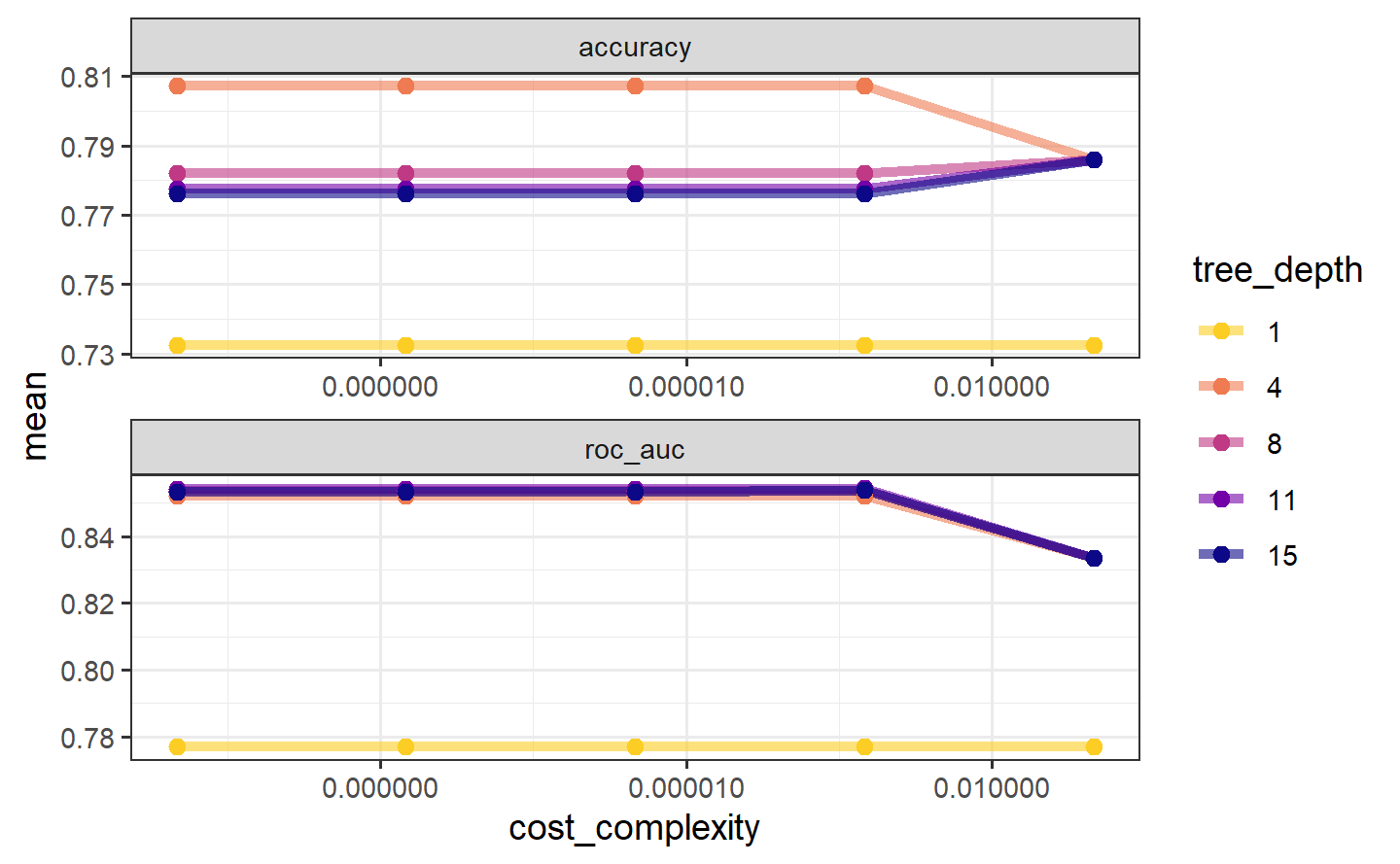

The show_best() function shows us the top 5 candidate models by default:

tree_res %>% 
  show_best("accuracy")
#> # A tibble: 5 × 8
#>   cost_complexity tree_depth .metric  .estimator  mean     n std_err .config    
#>             <dbl>      <int> <chr>    <chr>      <dbl> <int>   <dbl> <chr>      
#> 1    0.0000000001          4 accuracy binary     0.807    10  0.0119 Preprocess…
#> 2    0.0000000178          4 accuracy binary     0.807    10  0.0119 Preprocess…
#> 3    0.00000316            4 accuracy binary     0.807    10  0.0119 Preprocess…
#> 4    0.000562              4 accuracy binary     0.807    10  0.0119 Preprocess…
#> 5    0.1                   4 accuracy binary     0.786    10  0.0124 Preprocess…

We can also use the select_best() function to pull out the single set of hyperparameter values for our best decision tree model:

best_tree <- tree_res %>% 
  select_best("accuracy")

best_tree
#> # A tibble: 1 × 3
#>   cost_complexity tree_depth .config              
#>             <dbl>      <int> <chr>                
#> 1    0.0000000001          4 Preprocessor1_Model06

2.4.5 Finalizing our model

We can update (or “finalize”) our workflow object tree_wf with the values from select_best().

final_wf <- 
  tree_wf %>% 
  finalize_workflow(best_tree)

final_wf
#> ══ Workflow ════════════════════════════════════════════════════════════════════
#> Preprocessor: Formula
#> Model: decision_tree()
#> 
#> ── Preprocessor ────────────────────────────────────────────────────────────────
#> class ~ .
#> 
#> ── Model ───────────────────────────────────────────────────────────────────────
#> Decision Tree Model Specification (classification)
#> 
#> Main Arguments:
#>   cost_complexity = 1e-10
#>   tree_depth = 4
#> 
#> Computational engine: rpart

Our tuning is done!

2.4.6 The last fit

We can use the function last_fit() with our finalized model; this function fits the finalized model on the full training data set and evaluates the finalized model on the testing data.

final_fit <- 
  final_wf %>% 
  last_fit(cell_split)

final_fit %>% 
  collect_metrics()
#> # A tibble: 2 × 4
#>   .metric  .estimator .estimate .config             
#>   <chr>    <chr>          <dbl> <chr>               
#> 1 accuracy binary         0.802 Preprocessor1_Model1
#> 2 roc_auc  binary         0.840 Preprocessor1_Model1

final_fit %>% 
  collect_predictions() %>% 
  roc_curve(class, .pred_PS) %>% 
  autoplot()

The performance metrics from the test set indicate that we did not overfit during our tuning procedure.

The final_fit object contains a finalized, fitted workflow that you can use for predicting on new data or further understanding the results. You may want to extract this object, using one of the extract_ helper functions.

final_tree <- extract_workflow(final_fit)
final_tree
#> ══ Workflow [trained] ══════════════════════════════════════════════════════════
#> Preprocessor: Formula
#> Model: decision_tree()
#> 
#> ── Preprocessor ────────────────────────────────────────────────────────────────
#> class ~ .
#> 
#> ── Model ───────────────────────────────────────────────────────────────────────
#> n= 1514 
#> 
#> node), split, n, loss, yval, (yprob)
#>       * denotes terminal node
#> 
#>  1) root 1514 539 PS (0.64398943 0.35601057)  
#>    2) total_inten_ch_2< 41732.5 642  33 PS (0.94859813 0.05140187)  
#>      4) shape_p_2_a_ch_1>=1.251801 631  27 PS (0.95721078 0.04278922) *
#>      5) shape_p_2_a_ch_1< 1.251801 11   5 WS (0.45454545 0.54545455) *
#>    3) total_inten_ch_2>=41732.5 872 366 WS (0.41972477 0.58027523)  
#>      6) fiber_width_ch_1< 11.37318 406 160 PS (0.60591133 0.39408867)  
#>       12) avg_inten_ch_1< 145.4883 293  85 PS (0.70989761 0.29010239) *
#>       13) avg_inten_ch_1>=145.4883 113  38 WS (0.33628319 0.66371681)  
#>         26) total_inten_ch_3>=57919.5 33  10 PS (0.69696970 0.30303030) *
#>         27) total_inten_ch_3< 57919.5 80  15 WS (0.18750000 0.81250000) *
#>      7) fiber_width_ch_1>=11.37318 466 120 WS (0.25751073 0.74248927)  
#>       14) eq_ellipse_oblate_vol_ch_1>=1673.942 30   8 PS (0.73333333 0.26666667)  
#>         28) var_inten_ch_3>=41.10858 20   2 PS (0.90000000 0.10000000) *
#>         29) var_inten_ch_3< 41.10858 10   4 WS (0.40000000 0.60000000) *
#>       15) eq_ellipse_oblate_vol_ch_1< 1673.942 436  98 WS (0.22477064 0.77522936) *

final_tree %>% 
  extract_fit_engine() %>% 
  rpart.plot(roundint = FALSE)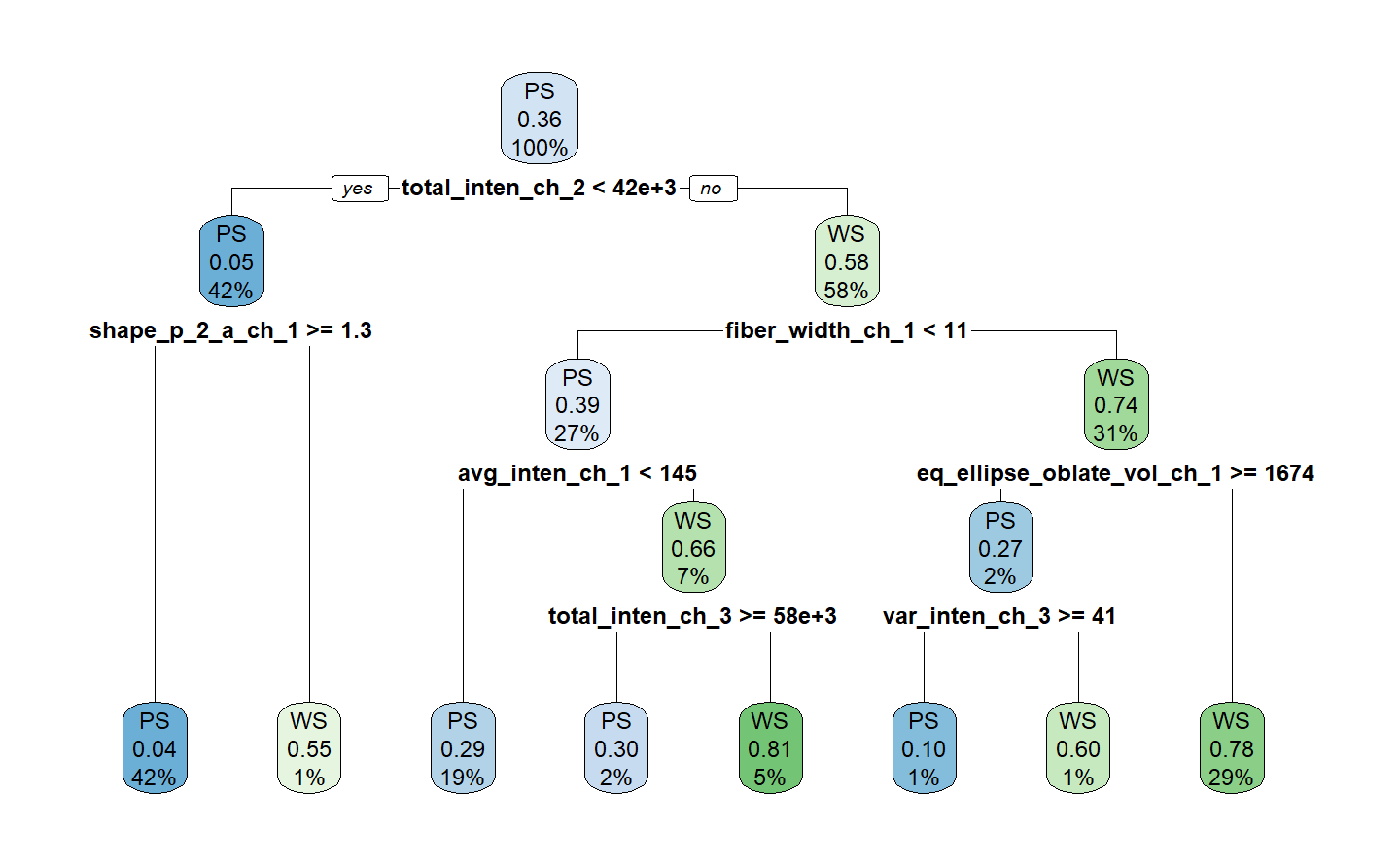

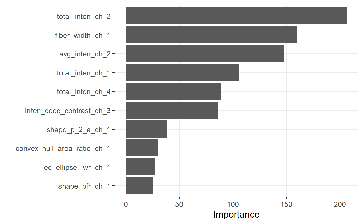
Perhaps we would also like to understand what variables are important in this final model. We can use the {vip} package to estimate variable importance based on the model’s structure.

final_tree %>% 
  extract_fit_parsnip() %>% 
  vip()

2.5 A predictive modeling case study

2.5.1 The hotel bookings data

hotels <- 
  read_csv("https://tidymodels.org/start/case-study/hotels.csv",
           show_col_types = FALSE) %>% 
  mutate(across(where(is.character), as_factor))

dim(hotels)
#> [1] 50000    23

glimpse(hotels)
#> Rows: 50,000
#> Columns: 23
#> $ hotel                          <fct> City_Hotel, City_Hotel, Resort_Hotel, R…
#> $ lead_time                      <dbl> 217, 2, 95, 143, 136, 67, 47, 56, 80, 6…
#> $ stays_in_weekend_nights        <dbl> 1, 0, 2, 2, 1, 2, 0, 0, 0, 2, 1, 0, 1, …
#> $ stays_in_week_nights           <dbl> 3, 1, 5, 6, 4, 2, 2, 3, 4, 2, 2, 1, 2, …
#> $ adults                         <dbl> 2, 2, 2, 2, 2, 2, 2, 0, 2, 2, 2, 1, 2, …
#> $ children                       <fct> none, none, none, none, none, none, chi…
#> $ meal                           <fct> BB, BB, BB, HB, HB, SC, BB, BB, BB, BB,…
#> $ country                        <fct> DEU, PRT, GBR, ROU, PRT, GBR, ESP, ESP,…
#> $ market_segment                 <fct> Offline_TA/TO, Direct, Online_TA, Onlin…
#> $ distribution_channel           <fct> TA/TO, Direct, TA/TO, TA/TO, Direct, TA…
#> $ is_repeated_guest              <dbl> 0, 0, 0, 0, 0, 0, 0, 0, 0, 0, 0, 0, 0, …
#> $ previous_cancellations         <dbl> 0, 0, 0, 0, 0, 0, 0, 0, 0, 0, 0, 0, 0, …
#> $ previous_bookings_not_canceled <dbl> 0, 0, 0, 0, 0, 0, 0, 0, 0, 0, 0, 0, 0, …
#> $ reserved_room_type             <fct> A, D, A, A, F, A, C, B, D, A, A, D, A, …
#> $ assigned_room_type             <fct> A, K, A, A, F, A, C, A, D, A, D, D, A, …
#> $ booking_changes                <dbl> 0, 0, 2, 0, 0, 0, 0, 0, 0, 0, 0, 0, 0, …
#> $ deposit_type                   <fct> No_Deposit, No_Deposit, No_Deposit, No_…
#> $ days_in_waiting_list           <dbl> 0, 0, 0, 0, 0, 0, 0, 0, 0, 0, 0, 0, 0, …
#> $ customer_type                  <fct> Transient-Party, Transient, Transient, …
#> $ average_daily_rate             <dbl> 80.75, 170.00, 8.00, 81.00, 157.60, 49.…
#> $ required_car_parking_spaces    <fct> none, none, none, none, none, none, non…
#> $ total_of_special_requests      <dbl> 1, 3, 2, 1, 4, 1, 1, 1, 1, 1, 0, 1, 0, …
#> $ arrival_date                   <date> 2016-09-01, 2017-08-25, 2016-11-19, 20…

2.5.2 Data splitting & resampling

set.seed(123)
splits <- initial_split(hotels, strata = children)

hotels_other <- training(splits)
hotel_test <- testing(splits)

# training set proportions by children
hotels_other %>% 
  count(children) %>% 
  mutate(prop = n / sum(n))
#> # A tibble: 2 × 3
#>   children     n   prop
#>   <fct>    <int>  <dbl>
#> 1 none     34473 0.919 
#> 2 children  3027 0.0807

# test set proportion by children
hotel_test %>% 
  count(children) %>% 
  mutate(prop = n / sum(n))
#> # A tibble: 2 × 3
#>   children     n   prop
#>   <fct>    <int>  <dbl>
#> 1 none     11489 0.919 
#> 2 children  1011 0.0809

For this case study, rather than using multiple iterations of resampling, let’s create a single resample called a validation set. In tidymodels, a validation set is treated as a single iteration of resampling. This will be a split from the 37,500 stays that were not used for testing, which we called hotel_other. This split creates two new datasets:

• the set held out for the purpose of measuring performance, called the validation set, and
• the remaining data used to fit the model, called the training set.

We’ll use the validation_split() function to allocate 20% of the hotel_other stays to the validation set and 30,000 stays to the training set. This means that our model performance metrics will be computed on a single set of 7,500 hotel stays. This is fairly large, so the amount of data should provide enough precision to be a reliable indicator for how well each model predicts the outcome with a single iteration of resampling.

set.seed(234)
val_set <- validation_split(hotels_other,
                            strata = children,
                            prop = .8)
val_set
#> # Validation Set Split (0.8/0.2)  using stratification 
#> # A tibble: 1 × 2
#>   splits               id        
#>   <list>               <chr>     
#> 1 <split [30000/7500]> validation

2.5.3 A first model: penalized logistic regression

# build the model
lr_mod <- 
  logistic_reg(penalty = tune(), mixture = 1) %>% 
  set_engine("glmnet")

Setting mixture to a value of one means that the glmnet model will potentially remove irrelevant predictors and choose a simpler model.

# create the recipe
holidays <- c("AllSouls", "AshWednesday", "ChristmasEve", 
              "Easter", "ChristmasDay", "GoodFriday",
              "NewYearsDay","PalmSunday")

lr_recipe <- 
  recipe(children ~ ., data = hotels_other) %>% 
  step_date(arrival_date) %>% 
  step_holiday(arrival_date, holidays = holidays) %>% 
  step_rm(arrival_date) %>% 
  step_dummy(all_nominal_predictors()) %>% 
  step_zv(all_predictors()) %>% 
  step_normalize(all_predictors())

# create the workflow
lr_wflow <- 
  workflow() %>% 
  add_model(lr_mod) %>% 
  add_recipe(lr_recipe)

# create the grid for tuning
lr_reg_grid <- tibble(penalty = 10^seq(-4, -1, length.out = 30))

Let’s use tune::tune_grid() to train these 30 penalized logistic regression models. We’ll also save the validation set predictions (via the call to control_grid()) so that diagnostic information can be available after the model fit. The area under the ROC curve will be used to quantify how well the model performs across a continuum of event thresholds (recall that the event rate—the proportion of stays including children— is very low for these data).

# train and tune the model
lr_res <- 
  lr_wflow %>% 
  tune_grid(val_set,
            grid = lr_reg_grid,
            control = control_grid(save_pred = TRUE),
            metrics = metric_set(roc_auc))

It might be easier to visualize the validation set metrics by plotting the area under the ROC curve against the range of penalty values:

lr_plot <- 
  lr_res %>% 
  collect_metrics() %>% 
  ggplot(aes(penalty, mean)) +
  geom_point() +
  geom_line() +
  ylab("Area under the ROC Curve") +
  scale_x_log10(labels = scales::label_number())

lr_plot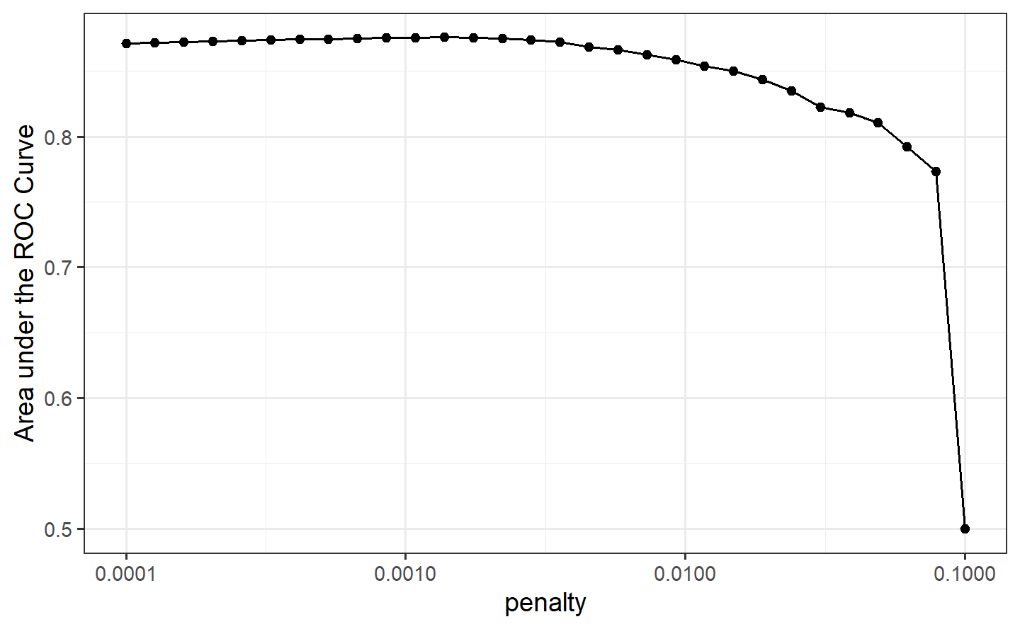

This plots shows us that model performance is generally better at the smaller penalty values. This suggests that the majority of the predictors are important to the model. We also see a steep drop in the area under the ROC curve towards the highest penalty values. This happens because a large enough penalty will remove all predictors from the model, and not surprisingly predictive accuracy plummets with no predictors in the model.

Our model performance seems to plateau at the smaller penalty values, so going by the roc_auc metric alone could lead us to multiple options for the “best” value for this hyperparameter:

top_models <- 
  lr_res %>% 
  show_best("roc_auc", n = 15) %>% 
  arrange(penalty)

top_models
#> # A tibble: 15 × 7
#>     penalty .metric .estimator  mean     n std_err .config              
#>       <dbl> <chr>   <chr>      <dbl> <int>   <dbl> <chr>                
#>  1 0.000127 roc_auc binary     0.872     1      NA Preprocessor1_Model02
#>  2 0.000161 roc_auc binary     0.872     1      NA Preprocessor1_Model03
#>  3 0.000204 roc_auc binary     0.873     1      NA Preprocessor1_Model04
#>  4 0.000259 roc_auc binary     0.873     1      NA Preprocessor1_Model05
#>  5 0.000329 roc_auc binary     0.874     1      NA Preprocessor1_Model06
#>  6 0.000418 roc_auc binary     0.874     1      NA Preprocessor1_Model07
#>  7 0.000530 roc_auc binary     0.875     1      NA Preprocessor1_Model08
#>  8 0.000672 roc_auc binary     0.875     1      NA Preprocessor1_Model09
#>  9 0.000853 roc_auc binary     0.875     1      NA Preprocessor1_Model10
#> 10 0.00108  roc_auc binary     0.876     1      NA Preprocessor1_Model11
#> 11 0.00137  roc_auc binary     0.876     1      NA Preprocessor1_Model12
#> 12 0.00174  roc_auc binary     0.876     1      NA Preprocessor1_Model13
#> 13 0.00221  roc_auc binary     0.875     1      NA Preprocessor1_Model14
#> 14 0.00281  roc_auc binary     0.874     1      NA Preprocessor1_Model15
#> 15 0.00356  roc_auc binary     0.872     1      NA Preprocessor1_Model16

However, we may want to choose a penalty value further along the x-axis, closer to where we start to see the decline in model performance. For example, candidate model 12 with a penalty value of 0.00174 has effectively the same performance as the numerically best model (model 11), but might eliminate more predictors. This penalty value is marked by the solid line above. In general, fewer irrelevant predictors is better. If performance is about the same, we’d prefer to choose a higher penalty value.

Let’s select this value and visualize the validation set ROC curve:

lr_best <- 
  lr_res %>% 
  collect_metrics() %>% 
  arrange(penalty) %>% 
  slice(12)

lr_best
#> # A tibble: 1 × 7
#>   penalty .metric .estimator  mean     n std_err .config              
#>     <dbl> <chr>   <chr>      <dbl> <int>   <dbl> <chr>                
#> 1 0.00137 roc_auc binary     0.876     1      NA Preprocessor1_Model12

lr_auc <- 
  lr_res %>% 
  collect_predictions(parameters = lr_best) %>% 
  roc_curve(children, .pred_none) %>% 
  mutate(model = "Logistic Regression")

autoplot(lr_auc)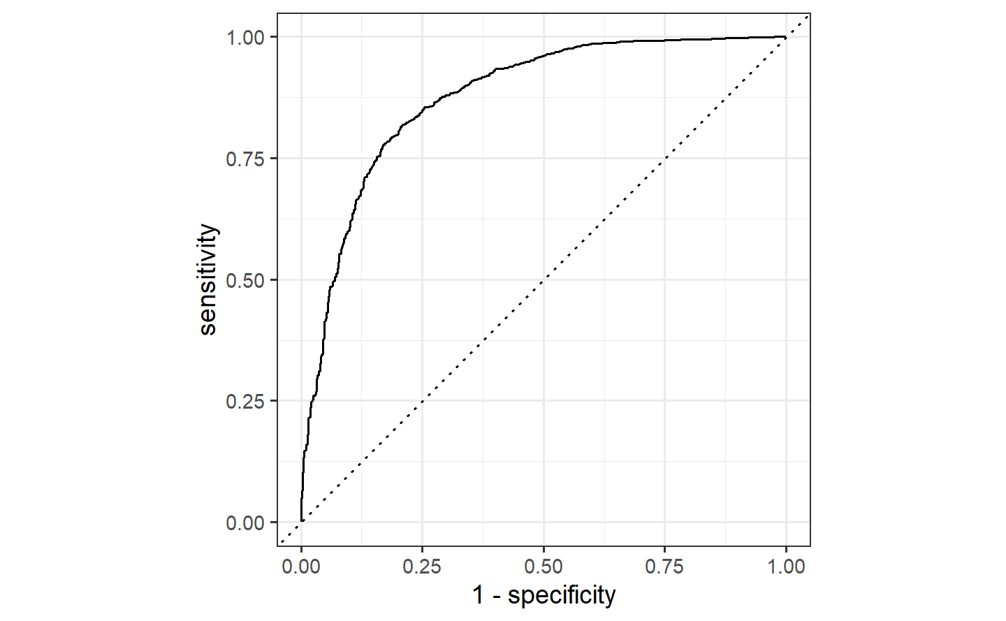

The level of performance generated by this logistic regression model is good, but not groundbreaking. Perhaps the linear nature of the prediction equation is too limiting for this data set. As a next step, we might consider a highly non-linear model generated using a tree-based ensemble method.

2.5.4 A second model: tree-based ensemble

Each tree is non-linear, and aggregating across trees makes random forests also non-linear but more robust and stable compared to individual trees. Tree-based models like random forests require very little preprocessing and can effectively handle many types of predictors (sparse, skewed, continuous, categorical, etc.).

Although the default hyperparameters for random forests tend to give reasonable results, we’ll plan to tune two hyperparameters that we think could improve performance. Unfortunately, random forest models can be computationally expensive to train and to tune. The computations required for model tuning can usually be easily parallelized to improve training time. The {tune} package can do parallel processing for you, and allows users to use multiple cores or separate machines to fit models.

But, here we are using a single validation set, so parallelization isn’t an option using the tune package. For this specific case study, a good alternative is provided by the engine itself. The {ranger} package offers a built-in way to compute individual random forest models in parallel. To do this, we need to know the the number of cores we have to work with. We can use the parallel package to query the number of cores on your own computer to understand how much parallelization you can do:

cores <- parallel::detectCores()
cores
#> [1] 8

We have 10 8 to work with. We can pass this information to the ranger engine when we set up our parsnip rand_forest() model. To enable parallel processing, we can pass engine-specific arguments like num.threads to ranger when we set the engine:

rf_mod <- 
  rand_forest(mtry = tune(), min_n = tune(), trees = 1000) %>% 
  set_engine("ranger", num.threads = cores) %>% 
  set_mode("classification")

This works well in this modeling context, but it bears repeating: if you use any other resampling method, let tune do the parallel processing for you — we typically do not recommend relying on the modeling engine (like we did here) to do this.

# create the recipe and workflow
rf_recipe <- 
  recipe(children ~ ., data = hotels_other) %>% 
  step_date(arrival_date) %>% 
  step_holiday(arrival_date) %>% 
  step_rm(arrival_date)

rf_wflow <- 
  workflow() %>% 
  add_model(rf_mod) %>% 
  add_recipe(rf_recipe)

# train and tune the model
rf_mod
#> Random Forest Model Specification (classification)
#> 
#> Main Arguments:
#>   mtry = tune()
#>   trees = 1000
#>   min_n = tune()
#> 
#> Engine-Specific Arguments:
#>   num.threads = cores
#> 
#> Computational engine: ranger

# show what will be tuned
extract_parameter_set_dials(rf_mod)
#> Collection of 2 parameters for tuning
#> 
#>  identifier  type    object
#>        mtry  mtry nparam[?]
#>       min_n min_n nparam[+]
#> 
#> Model parameters needing finalization:
#>    # Randomly Selected Predictors ('mtry')
#> 
#> See `?dials::finalize` or `?dials::update.parameters` for more information.

set.seed(345)
rf_res <- 
  rf_wflow %>% 
  tune_grid(val_set,
            grid = 25,
            control = control_grid(save_pred = TRUE),
            metrics = metric_set(roc_auc))
#> i Creating pre-processing data to finalize unknown parameter: mtry

The message printed above “Creating pre-processing data to finalize unknown parameter: mtry” is related to the size of the data set. Since mtry depends on the number of predictors in the data set, tune_grid() determines the upper bound for mtry once it receives the data.

rf_res %>% 
  show_best(metric = "roc_auc")
#> # A tibble: 5 × 8
#>    mtry min_n .metric .estimator  mean     n std_err .config              
#>   <int> <int> <chr>   <chr>      <dbl> <int>   <dbl> <chr>                
#> 1     8     7 roc_auc binary     0.925     1      NA Preprocessor1_Model13
#> 2     9    12 roc_auc binary     0.924     1      NA Preprocessor1_Model19
#> 3    13     4 roc_auc binary     0.924     1      NA Preprocessor1_Model05
#> 4     6    18 roc_auc binary     0.923     1      NA Preprocessor1_Model24
#> 5    12     7 roc_auc binary     0.923     1      NA Preprocessor1_Model01

autoplot(rf_res)

# select the best model
rf_best <- 
  rf_res %>% 
  select_best(metric = "roc_auc")

rf_best
#> # A tibble: 1 × 3
#>    mtry min_n .config              
#>   <int> <int> <chr>                
#> 1     8     7 Preprocessor1_Model13

To calculate the data needed to plot the ROC curve, we use collect_predictions(). This is only possible after tuning with control_grid(save_pred = TRUE). In the output, you can see the two columns that hold our class probabilities for predicting hotel stays including and not including children.

rf_res %>% 
  collect_predictions()
#> # A tibble: 187,500 × 8
#>    id         .pred_none .pred_children  .row  mtry min_n children .config      
#>    <chr>           <dbl>          <dbl> <int> <int> <int> <fct>    <chr>        
#>  1 validation      0.790       0.210       13    12     7 none     Preprocessor…
#>  2 validation      0.988       0.0117      20    12     7 none     Preprocessor…
#>  3 validation      0.536       0.464       22    12     7 children Preprocessor…
#>  4 validation      0.993       0.00737     23    12     7 none     Preprocessor…
#>  5 validation      0.988       0.0118      31    12     7 none     Preprocessor…
#>  6 validation      0.999       0.000843    38    12     7 none     Preprocessor…
#>  7 validation      1           0           39    12     7 none     Preprocessor…
#>  8 validation      0.991       0.00899     50    12     7 none     Preprocessor…
#>  9 validation      0.974       0.0262      54    12     7 none     Preprocessor…
#> 10 validation      0.958       0.0423      57    12     7 children Preprocessor…
#> # ℹ 187,490 more rows

To filter the predictions for only our best random forest model, we can use the parameters argument and pass it our tibble with the best hyperparameter values from tuning, which we called rf_best:

rf_auc <- 
  rf_res %>% 
  collect_predictions(parameters = rf_best) %>% 
  roc_curve(children, .pred_none) %>% 
  mutate(model = "Random Forest")

Now, we can compare the validation set ROC curves for our top penalized logistic regression model and random forest model:

bind_rows(rf_auc, lr_auc) %>% 
  ggplot(aes(x = 1 - specificity, y = sensitivity,
             col = model)) +
  geom_path(lwd = 1.5, alpha = .8) +
  geom_abline(lty = 3) +
  coord_equal() +
  scale_color_viridis_d(option = "plasma", end = .6)

The random forest is uniformly better across event probability thresholds.

2.5.5 The last fit

After selecting our best model and hyperparameter values, our last step is to fit the final model on all the rows of data not originally held out for testing (both the training and the validation sets combined), and then evaluate the model performance one last time with the held-out test set.

We’ll start by building our parsnip model object again from scratch. We take our best hyperparameter values from our random forest model. When we set the engine, we add a new argument: importance = "impurity". This will provide variable importance scores for this last model, which gives some insight into which predictors drive model performance.

# the last model
last_rf_mod <- 
  rand_forest(mtry = 8, min_n = 7, trees = 1000) %>% 
  set_engine("ranger", num.threads = cores, importance = "impurity") %>% 
  set_mode("classification")

# the last workflow
last_rf_wflow <- 
  rf_wflow %>% 
  update_model(last_rf_mod)

# the last fit
set.seed(345)
last_rf_fit <- 
  last_rf_wflow %>% 
  last_fit(splits)

last_rf_fit
#> # Resampling results
#> # Manual resampling 
#> # A tibble: 1 × 6
#>   splits                id             .metrics .notes   .predictions .workflow 
#>   <list>                <chr>          <list>   <list>   <list>       <list>    
#> 1 <split [37500/12500]> train/test sp… <tibble> <tibble> <tibble>     <workflow>

This fitted workflow contains everything, including our final metrics based on the test set. So, how did this model do on the test set? Was the validation set a good estimate of future performance?

last_rf_fit %>% 
  collect_metrics()
#> # A tibble: 2 × 4
#>   .metric  .estimator .estimate .config             
#>   <chr>    <chr>          <dbl> <chr>               
#> 1 accuracy binary         0.947 Preprocessor1_Model1
#> 2 roc_auc  binary         0.925 Preprocessor1_Model1

This ROC AUC value is pretty close to what we saw when we tuned the random forest model with the validation set, which is good news. That means that our estimate of how well our model would perform with new data was not too far off from how well our model actually performed with the unseen test data.

We can access those variable importance scores via the .workflow column. We can extract out the fit from the workflow object, and then use the vip package to visualize the variable importance scores for the top 20 features:

last_rf_fit %>% 
  extract_fit_parsnip() %>% 
  vip(num_features = 20)

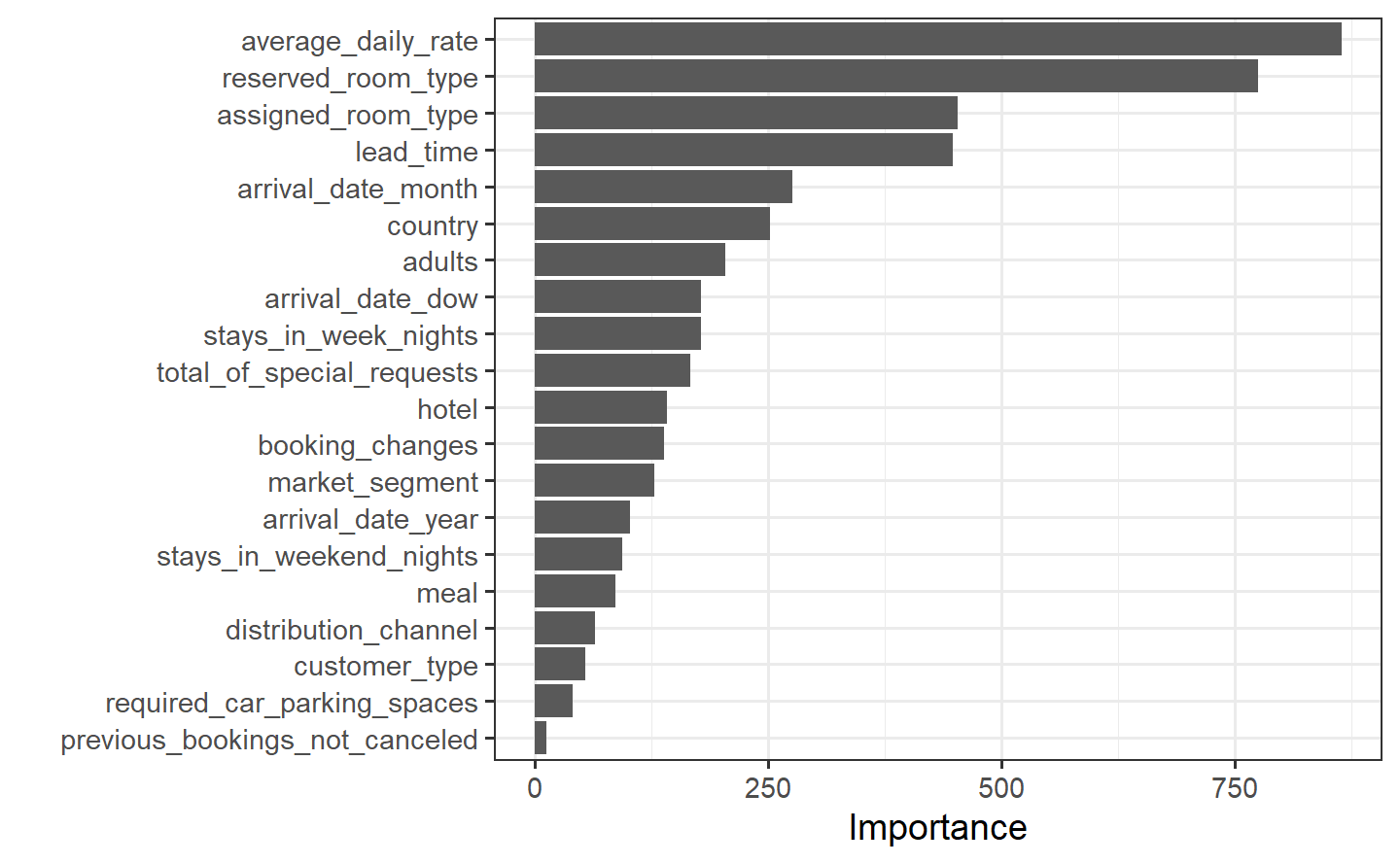
The most important predictors in whether a hotel stay had children or not were the daily cost for the room, the type of room reserved, the time between the creation of the reservation and the arrival date, and the type of room that was ultimately assigned.

last_rf_fit %>% 
  collect_predictions() %>% 
  roc_curve(children, .pred_none) %>% 
  autoplot()

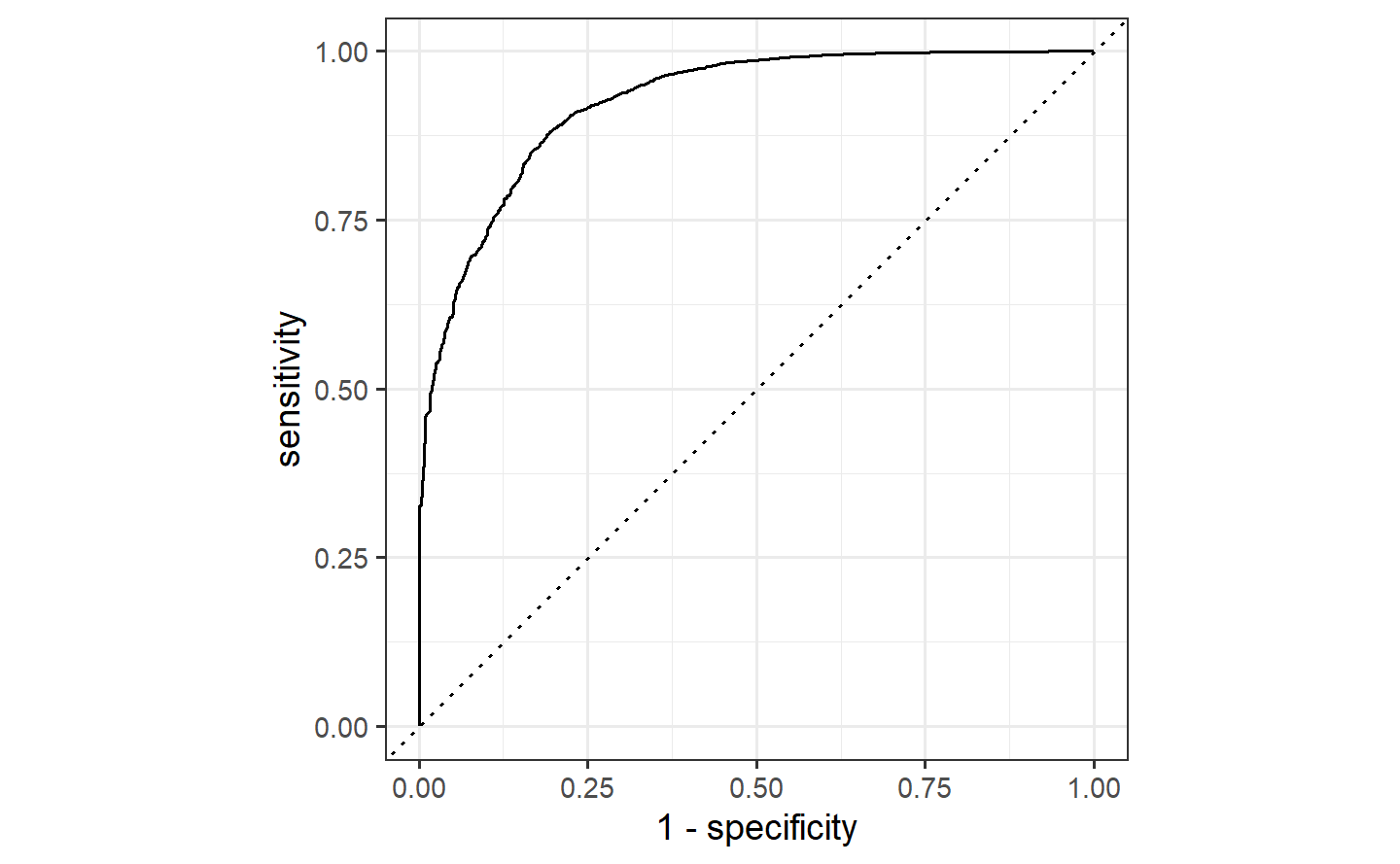
Based on these results, the validation set and test set performance statistics are very close, so we would have pretty high confidence that our random forest model with the selected hyperparameters would perform well when predicting new data.