Progress

Learning Progress: Paused, current progress 75.76%.⏱

Learning Source

https://jakevdp.github.io/PythonDataScienceHandbook/

1 IPython Beyond Normal Python

1.1 Help and Documentation in IPython

If you play with this much, you’ll notice that sometimes the ?? suffix doesn’t display any source code: this is generally because the object in question is not implemented in Python, but in C or some other compiled extension language. If this is the case, the ?? suffix gives the same output as the ? suffix. You’ll find this particularly with many of Python’s built-in objects and types.
Though Python has no strictly enforced distinction between public/external attributes and private/internal attributes, by convention a preceding underscore is used to denote the latter. For clarity, these private methods and special methods are omitted from the list by default, but it’s possible to list them by explicitly typing the underscore.

1.2 IPython Magic Commands

As you begin developing more extensive code, you will likely find yourself working in IPython for interactive exploration, as well as a text editor to store code that you want to reuse. Rather than running this code in a new window, it can be convenient to run it within your IPython session. This can be done with the %run magic command.

# file: myscript.py
%run myscript.py

1 squared is 1
2 squared is 4
3 squared is 9

Another example of a useful magic function is %timeit, which will automatically determine the execution time of the single-line Python statement that follows it. For example, we may want to check the performance of a list comprehension:

%timeit L = [n ** 2 for n in range(1000)]

75.6 µs ± 2.93 µs per loop (mean ± std. dev. of 7 runs, 10,000 loops each)

%%timeit
L = []
for n in range(1000):
    L.append(n ** 2)

85.2 µs ± 1.55 µs per loop (mean ± std. dev. of 7 runs, 10,000 loops each)

Like normal Python functions, IPython magic functions have docstrings, and this useful documentation can be accessed in the standard manner. So, for example, to read the documentation of the %timeit magic function, simply type this:

%timeit?

1.3 Input and Output History

The standard Python shell contains just one simple shortcut for accessing previous output: the variable _ (i.e., a single underscore) is kept updated with the previous output. This works in IPython as well. But IPython takes this a bit further—you can use a double underscore to access the second-to-last output, and a triple underscore to access the third-to-last output (skipping any commands with no output). IPython stops there: more than three underscores starts to get a bit hard to count, and at that point it’s easier to refer to the output by line number.

There is one more shortcut I should mention, however—a shorthand for Out[X] is _X (i.e., a single underscore followed by the line number):

_2

Sometimes you might wish to suppress the output of a statement, or maybe the command you’re executing produces a result that you’d prefer not to store in your output history, perhaps so that it can be deallocated when other references are removed. The easiest way to suppress the output of a command is to add a semicolon to the end of the line:

import math

math.sin(2) + math.cos(2);

The result is computed silently, and the output is neither displayed on the screen nor stored in the Out dictionary:

14 in Out

2 Introduction to NumPy

import numpy as np

np.__version__

'1.26.1'

2.1 Understanding Data Types in Python

2.1.1 A Python List Is More Than Just a List

At the implementation level, the array essentially contains a single pointer to one contiguous block of data. The Python list, on the other hand, contains a pointer to a block of pointers, each of which in turn points to a full Python object like the Python integer we saw earlier. Again, the advantage of the list is flexibility: because each list element is a full structure containing both data and type information, the list can be filled with data of any desired type. Fixed-type NumPy-style arrays lack this flexibility, but are much more efficient for storing and manipulating data.

2.1.2 Creating Arrays from Python Lists

# Integer array
np.array([1, 4, 2, 5, 3])

array([1, 4, 2, 5, 3])

# Integer upcast to floating point
np.array([3.14, 3, 2, 3])

array([3.14, 3.  , 2.  , 3.  ])

# Set data type
np.array([1, 2, 3, 4], dtype = np.float32)

array([1., 2., 3., 4.], dtype=float32)

NumPy arrarys can be multidimensional:

# Nested list result in multidismentional arrays
np.array([range(i, i + 3) for i in [2, 4, 6]])

array([[2, 3, 4],
       [4, 5, 6],
       [6, 7, 8]])

2.1.3 Creating Arrays from Scratch

# Create a length-10 integer array filled with 0s
np.zeros(10, dtype = int)

array([0, 0, 0, 0, 0, 0, 0, 0, 0, 0])

# Create a 3x5 floating-point array filled with 1s
np.ones((3, 5), dtype = float)

array([[1., 1., 1., 1., 1.],
       [1., 1., 1., 1., 1.],
       [1., 1., 1., 1., 1.]])

# Create a 3x5 array filled with 3.14
np.full((3, 5), 3.14)

array([[3.14, 3.14, 3.14, 3.14, 3.14],
       [3.14, 3.14, 3.14, 3.14, 3.14],
       [3.14, 3.14, 3.14, 3.14, 3.14]])

# Create an array filled with a linear sequence
np.arange(0, 20, 2)

array([ 0,  2,  4,  6,  8, 10, 12, 14, 16, 18])

# Create an array of five values evenly spaced between 0 and 1
np.linspace(0, 1, 5)

array([0.  , 0.25, 0.5 , 0.75, 1.  ])

# Create a 3x3 array of uniformly distributed pseudorandom
# values between 0 and 1
np.random.random((3, 3))

array([[0.25929357, 0.22696949, 0.89157503],
       [0.81186656, 0.44812646, 0.88065959],
       [0.94284462, 0.1762824 , 0.59956876]])

# Create a 3x3 array of normally distributed pseudorandom
# values with mean 0 and standard deviation 1
np.random.normal(0, 1, (3, 3))

array([[ 0.51180277,  0.1152987 , -0.68647798],
       [ 0.77800191,  0.3676049 ,  1.03042757],
       [ 0.38366847,  0.11996074, -0.9047977 ]])

# Create a 3x3 array of pseudorandom integers in the interval [0, 10)
np.random.randint(0, 10, (3, 3))

array([[4, 1, 7],
       [3, 6, 4],
       [7, 7, 4]])

# Create a 3x3 identity matrix
np.eye(3)

array([[1., 0., 0.],
       [0., 1., 0.],
       [0., 0., 1.]])

# Create an uninitialized array of three integers; the values will be
# whatever happens to already exist at that memory location
np.empty(3)

array([1., 1., 1.])

2.2 The Basics of NumPy Arrays

np.random.seed(0)

x1 = np.random.randint(10, size = 6)
x2 = np.random.randint(10, size = (3, 4))
x3 = np.random.randint(10, size = (3, 4, 5))

Each array has attributes ndim (the number of dimensions), shape (the size of each dimension), and size (the total size of the array):

print("x3 ndim: ", x3.ndim)
print("x3 shape: ", x3.shape)
print("x3 size: ", x3.size)

x3 ndim:  3
x3 shape:  (3, 4, 5)
x3 size:  60

3 Machine Learning

3.1 What Is Machine Learning?

Fundamentally, machine learning involves building mathematical models to help understand data. “Learning” enters the fray when we give these models tunable parameters that can be adapted to observed data; in this way the program can be considered to be “learning” from the data. Once these models have been fit to previously seen data, they can be used to predict and understand aspects of newly observed data.1

3.2 Introducing Scikit-Learn

3.2.1 Data Representation in Scikit-Learn

import seaborn as sns
iris = sns.load_dataset('iris')
iris.head()

	sepal_length	sepal_width	petal_length	petal_width	species
0	5.1	3.5	1.4	0.2	setosa
1	4.9	3.0	1.4	0.2	setosa
2	4.7	3.2	1.3	0.2	setosa
3	4.6	3.1	1.5	0.2	setosa
4	5.0	3.6	1.4	0.2	setosa

%matplotlib inline
sns.set()
sns.pairplot(iris, hue = 'species', size = 1.5)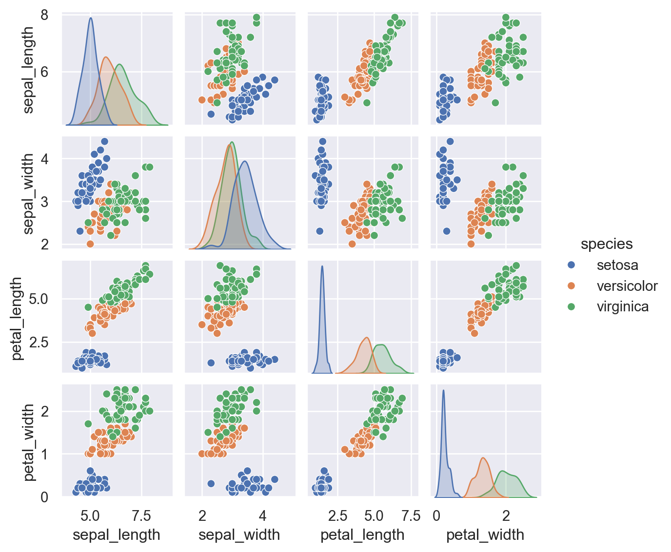

X_iris = iris.drop("species", axis = 1)
X_iris.shape

(150, 4)

y_iris = iris["species"]
y_iris.shape

(150,)

3.2.2 Scikit-Learn’s Estimator API

3.2.2.1 Supervised learning example: Simple linear regression

import matplotlib.pyplot as plt
import numpy as np

rng = np.random.RandomState(42)
x = 10 * rng.rand(50)
y = 2 * x - 1 + rng.randn(50)
plt.scatter(x, y)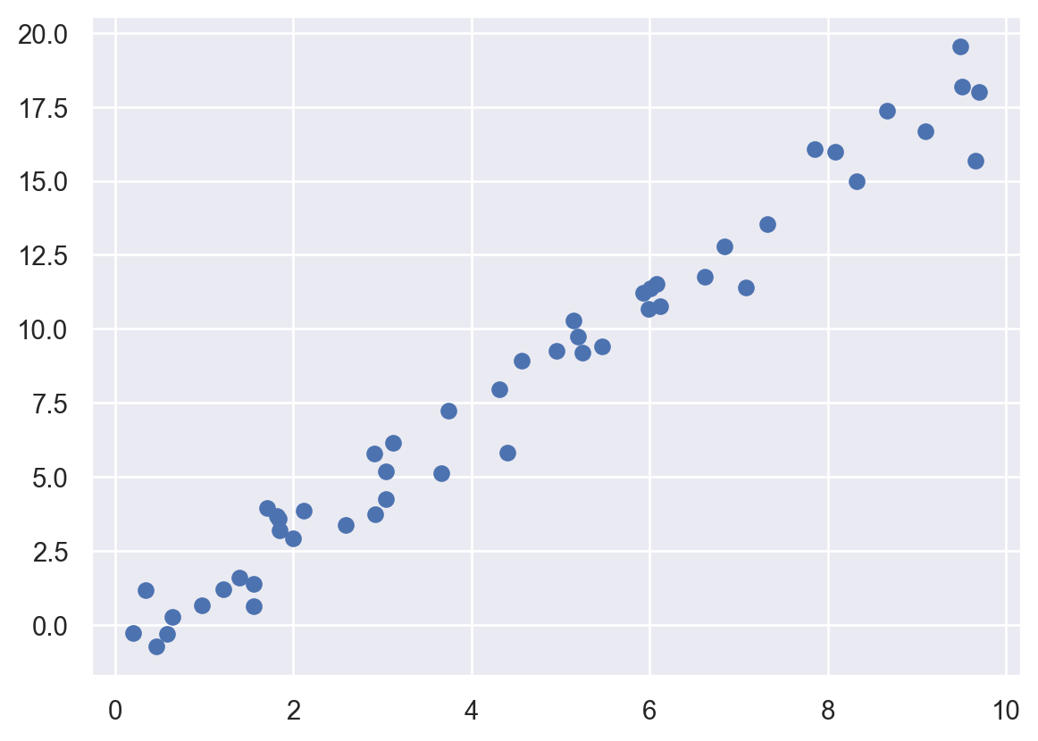

import sklearn
from sklearn.linear_model import LinearRegression

An important point is that a class of model is not the same as an instance of a model.

model = LinearRegression(fit_intercept = True)
model

LinearRegression()

In a Jupyter environment, please rerun this cell to show the HTML representation or trust the notebook.
On GitHub, the HTML representation is unable to render, please try loading this page with nbviewer.org.

Keep in mind that when the model is instantiated, the only action is the storing of these hyperparameter values. In particular, we have not yet applied the model to any data: the Scikit-Learn API makes very clear the distinction between choice of model and application of model to data.

# Arrange data into a features matrix and target vector
X = x[:, np.newaxis]
X.shape

(50, 1)

# Fit the model to your data
model.fit(X, y)

LinearRegression()

In Scikit-Learn, by convention all model parameters that were learned during the fit() process have trailing underscores; for example in this linear model, we have the following:

model.coef_

array([1.9776566])

model.intercept_

-0.903310725531111

# Predict labels for unknown data
xfit = np.linspace(-1, 11)
Xfit = xfit[:, np.newaxis]
yfit = model.predict(Xfit)

plt.scatter(x, y)
plt.plot(xfit, yfit)

3.3 Hyperparameters and Model Validation

To be continued

https://jakevdp.github.io/PythonDataScienceHandbook/05.03-hyperparameters-and-model-validation.html